Black-body radiation is the type of electromagnetic radiation within or surrounding a body in thermodynamic equilibrium with its environment, or emitted by a black body (an opaque and non-reflective body) held at constant, uniform temperature. The radiation has a specific spectrum and intensity that depends only on the temperature of the body.
A black-body at room temperature appears black, as most of the energy it radiates is infra-red and cannot be perceived by the human eye. At higher temperatures, black bodies glow with increasing intensity and colors that range from dull red to blindingly brilliant blue-white as the temperature increases.
The Black Body Ultraviolet Catastrophe Experiment
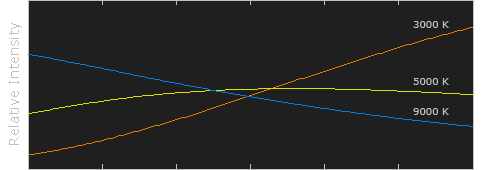
In photography, color temperature describes the spectrum of light which is radiated from a “blackbody” with that surface temperature. A blackbody is an object which absorbs all incident light — neither reflecting it nor allowing it to pass through.
The Sun closely approximates a black-body radiator. Another rough analogue of blackbody radiation in our day to day experience might be in heating a metal or stone: these are said to become “red hot” when they attain one temperature, and then “white hot” for even higher temperatures. Similarly, black bodies at different temperatures also have varying color temperatures of “white light.”
Despite its name, light which may appear white does not necessarily contain an even distribution of colors across the visible spectrum.
Although planets and stars are neither in thermal equilibrium with their surroundings nor perfect black bodies, black-body radiation is used as a first approximation for the energy they emit. Black holes are near-perfect black bodies, and it is believed that they emit black-body radiation (called Hawking radiation), with a temperature that depends on the mass of the hole.
In video terms gamut is normally related to as the full range of colours and brightness that can be either captured or displayed.
Generally speaking all color gamuts recommendations are trying to define a reasonable level of color representation based on available technology and hardware. REC-601 represents the old TVs. REC-709 is currently the most distributed solution. P3 is mainly available in movie theaters and is now being adopted in some of the best new 4K HDR TVs. Rec2020 (a wider space than P3 that improves on visibke color representation) and ACES (the full coverage of visible color) are other common standards which see major hardware development these days.
To compare and visualize different solution (across video and printing solutions), most developers use the CIE color model chart as a reference.
The CIE color model is a color space model created by the International Commission on Illumination known as the Commission Internationale de l’Elcairage (CIE) in 1931. It is also known as the CIE XYZ color space or the CIE 1931 XYZ color space.
This chart represents the first defined quantitative link between distributions of wavelengths in the electromagnetic visible spectrum, and physiologically perceived colors in human color vision. Or basically, the range of color a typical human eye can perceive through visible light.
Note that while the human perception is quite wide, and generally speaking biased towards greens (we are apes after all), the amount of colors available through nature, generated through light reflection, tend to be a much smaller section. This is defined by the Pointer’s Chart.
In short. Color gamut is a representation of color coverage, used to describe data stored in images against available hardware and viewer technologies.
The CIE 1931 standard has been replaced by a CIE 1976 standard. Below we can see the significance of this.
People have observed that the biggest issue with CIE 1931 is the lack of uniformity with chromaticity, the three dimension color space in rectangular coordinates is not visually uniformed.
The CIE 1976 (also called CIELUV) was created by the CIE in 1976. It was put forward in an attempt to provide a more uniform color spacing than CIE 1931 for colors at approximately the same luminance
The CIE 1976 standard colour space is more linear and variations in perceived colour between different people has also been reduced. The disproportionately large green-turquoise area in CIE 1931, which cannot be generated with existing computer screens, has been reduced.
If we move from CIE 1931 to the CIE 1976 standard colour space we can see that the improvements made in the gamut for the “new” iPad screen (as compared to the “old” iPad 2) are more evident in the CIE 1976 colour space than in the CIE 1931 colour space, particularly in the blues from aqua to deep blue.
Despite its age, CIE 1931, named for the year of its adoption, remains a well-worn and familiar shorthand throughout the display industry. CIE 1931 is the primary language of customers. When a customer says that their current display “can do 72% of NTSC,” they implicitly mean 72% of NTSC 1953 color gamut as mapped against CIE 1931.
An exposure stop is a unit measurement of Exposure as such it provides a universal linear scale to measure the increase and decrease in light, exposed to the image sensor, due to changes in shutter speed, iso and f-stop.
+-1 stop is a doubling or halving of the amount of light let in when taking a photo
1 EV (exposure value) is just another way to say one stop of exposure change.
Same applies to shutter speed, iso and aperture.
Doubling or halving your shutter speed produces an increase or decrease of 1 stop of exposure.
Doubling or halving your iso speed produces an increase or decrease of 1 stop of exposure.
“a simple yet effective technique to estimate lighting in a single input image. Current techniques rely heavily on HDR panorama datasets to train neural networks to regress an input with limited field-of-view to a full environment map. However, these approaches often struggle with real-world, uncontrolled settings due to the limited diversity and size of their datasets. To address this problem, we leverage diffusion models trained on billions of standard images to render a chrome ball into the input image. Despite its simplicity, this task remains challenging: the diffusion models often insert incorrect or inconsistent objects and cannot readily generate images in HDR format. Our research uncovers a surprising relationship between the appearance of chrome balls and the initial diffusion noise map, which we utilize to consistently generate high-quality chrome balls. We further fine-tune an LDR difusion model (Stable Diffusion XL) with LoRA, enabling it to perform exposure bracketing for HDR light estimation. Our method produces convincing light estimates across diverse settings and demonstrates superior generalization to in-the-wild scenarios.”
import math,sys

def Exposure2Intensity(exposure):
    exp = float(exposure)
    result = math.pow(2,exp)
    print(result)

Exposure2Intensity(0)

def Intensity2Exposure(intensity):
    inarg = float(intensity)

    if inarg == 0:
        print("Exposure of zero intensity is undefined.")
        return

    if inarg < 1e-323:
        inarg = max(inarg, 1e-323)
        print("Exposure of negative intensities is undefined. Clamping to a very small value instead (1e-323)")

    result = math.log(inarg, 2)
    print(result)

Intensity2Exposure(0.1)
Why Exposure?
Exposure is a stop value that multiplies the intensity by 2 to the power of the stop. Increasing exposure by 1 results in double the amount of light.
Artists think in “stops.” Doubling or halving brightness is easy math and common in grading and look-dev. Exposure counts doublings in whole stops:
+1 stop = ×2 brightness
−1 stop = ×0.5 brightness
This gives perceptually even controls across both bright and dark values.
Why Intensity?
Intensity is linear. It’s what render engines and compositors expect when:
Summing values
Averaging pixels
Multiplying or filtering pixel data
Use intensity when you need the actual math on pixel/light data.
Formulas (from your Python)
Intensity from exposure: intensity = 2**exposure
Exposure from intensity: exposure = log₂(intensity)
Guardrails:
Intensity must be > 0 to compute exposure.
If intensity = 0 → exposure is undefined.
Clamp tiny values (e.g. 1e−323) before using log₂.
Use Exposure (stops) when…
You want artist-friendly sliders (−5…+5 stops)
Adjusting look-dev or grading in even stops
Matching plates with quick ±1 stop tweaks
Tweening brightness changes smoothly across ranges
Use Intensity (linear) when…
Storing raw pixel/light values
Multiplying textures or lights by a gain
Performing sums, averages, and filters
Feeding values to render engines expecting linear data
Examples
+2 stops → 2**2 = 4.0 (×4)
+1 stop → 2**1 = 2.0 (×2)
0 stop → 2**0 = 1.0 (×1)
−1 stop → 2**(−1) = 0.5 (×0.5)
−2 stops → 2**(−2) = 0.25 (×0.25)
Intensity 0.1 → exposure = log₂(0.1) ≈ −3.32
Rule of thumb
Think in stops (exposure) for controls and matching. Compute in linear (intensity) for rendering and math.
Physically-based shading means leaving behind phenomenological models, like the Phong shading model, which are simply built to “look good” subjectively without being based on physics in any real way, and moving to lighting and shading models that are derived from the laws of physics and/or from actual measurements of the real world, and rigorously obey physical constraints such as energy conservation.
For example, in many older rendering systems, shading models included separate controls for specular highlights from point lights and reflection of the environment via a cubemap. You could create a shader with the specular and the reflection set to wildly different values, even though those are both instances of the same physical process. In addition, you could set the specular to any arbitrary brightness, even if it would cause the surface to reflect more energy than it actually received.
In a physically-based system, both the point light specular and the environment reflection would be controlled by the same parameter, and the system would be set up to automatically adjust the brightness of both the specular and diffuse components to maintain overall energy conservation. Moreover you would want to set the specular brightness to a realistic value for the material you’re trying to simulate, based on measurements.
Physically-based lighting or shading includes physically-based BRDFs, which are usually based on microfacet theory, and physically correct light transport, which is based on the rendering equation (although heavily approximated in the case of real-time games).
It also includes the necessary changes in the art process to make use of these features. Switching to a physically-based system can cause some upsets for artists. First of all it requires full HDR lighting with a realistic level of brightness for light sources, the sky, etc. and this can take some getting used to for the lighting artists. It also requires texture/material artists to do some things differently (particularly for specular), and they can be frustrated by the apparent loss of control (e.g. locking together the specular highlight and environment reflection as mentioned above; artists will complain about this). They will need some time and guidance to adapt to the physically-based system.
On the plus side, once artists have adapted and gained trust in the physically-based system, they usually end up liking it better, because there are fewer parameters overall (less work for them to tweak). Also, materials created in one lighting environment generally look fine in other lighting environments too. This is unlike more ad-hoc models, where a set of material parameters might look good during daytime, but it comes out ridiculously glowy at night, or something like that.
Here are some resources to look at for physically-based lighting in games:
SIGGRAPH 2013 Physically Based Shading Course, particularly the background talk by Naty Hoffman at the beginning. You can also check out the previous incarnations of this course for more resources.
And of course, I would be remiss if I didn’t mention Physically-Based Rendering by Pharr and Humphreys, an amazing reference on this whole subject and well worth your time, although it focuses on offline rather than real-time rendering.
Bella works in spectral space, allowing effects such as BSDF wavelength dependency, diffraction, or atmosphere to be modeled far more accurately than in color space.
IES profiles are useful for creating life-like lighting, as they can represent the physical distribution of light from any light source.
The IES format was created by the Illumination Engineering Society, and most lighting manufacturers provide IES profile for the lights they manufacture.
DISCLAIMER – Links and images on this website may be protected by the respective owners’ copyright. All data submitted by users through this site shall be treated as freely available to share.


