Depth of field is the range within which focusing is resolved in a photo.
Aperture has a huge affect on to the depth of field.
Changing the f-stops (f/#) of a lens will change aperture and as such the DOF.
f-stops are a just certain number which is telling you the size of the aperture. That’s how f-stop is related to aperture (and DOF).
If you increase f-stops, it will increase DOF, the area in focus (and decrease the aperture). On the other hand, decreasing the f-stop it will decrease DOF (and increase the aperture).
The red cone in the figure is an angular representation of the resolution of the system. Versus the dotted lines, which indicate the aperture coverage. Where the lines of the two cones intersect defines the total range of the depth of field.
This image explains why the longer the depth of field, the greater the range of clarity.
The intricate relationship between the eyes and the brain, often termed the eye-mind connection, reveals that vision is predominantly a cognitive process. This understanding has profound implications for fields such as design, where capturing and maintaining attention is paramount. This essay delves into the nuances of visual perception, the brain’s role in interpreting visual data, and how this knowledge can be applied to effective design strategies.
This cognitive aspect of vision is evident in phenomena such as optical illusions, where the brain interprets visual information in a way that contradicts physical reality. These illusions underscore that what we “see” is not merely a direct recording of the external world but a constructed experience shaped by cognitive processes.
Understanding the cognitive nature of vision is crucial for effective design. Designers must consider how the brain processes visual information to create compelling and engaging visuals. This involves several key principles:
Since spending a lot of time recently with SDXL I’ve since made my way back to SD 1.5
While the models overall have less fidelity. There is just no comparing to the current motion models we have available for animatediff with 1.5 models.
To date this is one of my favorite pieces. Not because I think it’s even the best it can be. But because the workflow adjustments unlocked some very important ideas I can’t wait to try out.
Performance by @silkenkelly and @itxtheballerina on IG
Spectral sensitivity of eye is influenced by light intensity. And the light intensity determines the level of activity of cones cell and rod cell. This is the main characteristic of human vision. Sensitivity to individual colors, in other words, wavelengths of the light spectrum, is explained by the RGB (red-green-blue) theory. This theory assumed that there are three kinds of cones. It’s selectively sensitive to red (700-630 nm), green (560-500 nm), and blue (490-450 nm) light. And their mutual interaction allow to perceive all colors of the spectrum.
One problem with sRGB is that in a gradient between blue and white, it becomes a bit purple in the middle of the transition. That’s because sRGB really isn’t created to mimic how the eye sees colors; rather, it is based on how CRT monitors work. That means it works with certain frequencies of red, green, and blue, and also the non-linear coding called gamma. It’s a miracle it works as well as it does, but it’s not connected to color perception. When using those tools, you sometimes get surprising results, like purple in the gradient.
There were also attempts to create simple models matching human perception based on XYZ, but as it turned out, it’s not possible to model all color vision that way. Perception of color is incredibly complex and depends, among other things, on whether it is dark or light in the room and the background color it is against. When you look at a photograph, it also depends on what you think the color of the light source is. The dress is a typical example of color vision being very context-dependent. It is almost impossible to model this perfectly.
I based Oklab on two other color spaces, CIECAM16 and IPT. I used the lightness and saturation prediction from CIECAM16, which is a color appearance model, as a target. I actually wanted to use the datasets used to create CIECAM16, but I couldn’t find them.
IPT was designed to have better hue uniformity. In experiments, they asked people to match light and dark colors, saturated and unsaturated colors, which resulted in a dataset for which colors, subjectively, have the same hue. IPT has a few other issues but is the basis for hue in Oklab.
In the Munsell color system, colors are described with three parameters, designed to match the perceived appearance of colors: Hue, Chroma and Value. The parameters are designed to be independent and each have a uniform scale. This results in a color solid with an irregular shape. The parameters are designed to be independent and each have a uniform scale. This results in a color solid with an irregular shape. Modern color spaces and models, such as CIELAB, Cam16 and Björn Ottosson own Oklab, are very similar in their construction.
By far the most used color spaces today for color picking are HSL and HSV, two representations introduced in the classic 1978 paper “Color Spaces for Computer Graphics”. HSL and HSV designed to roughly correlate with perceptual color properties while being very simple and cheap to compute.
Today HSL and HSV are most commonly used together with the sRGB color space.
One of the main advantages of HSL and HSV over the different Lab color spaces is that they map the sRGB gamut to a cylinder. This makes them easy to use since all parameters can be changed independently, without the risk of creating colors outside of the target gamut.
The main drawback on the other hand is that their properties don’t match human perception particularly well.
Reconciling these conflicting goals perfectly isn’t possible, but given that HSV and HSL don’t use anything derived from experiments relating to human perception, creating something that makes a better tradeoff does not seem unreasonable.
With this new lightness estimate, we are ready to look into the construction of Okhsv and Okhsl.
About 576 megapixels for the entire field of view.
Consider a view in front of you that is 90 degrees by 90 degrees, like looking through an open window at a scene. The number of pixels would be:
90 degrees * 60 arc-minutes/degree * 1/0.3 * 90 * 60 * 1/0.3 = 324,000,000 pixels (324 megapixels).
At any one moment, you actually do not perceive that many pixels, but your eye moves around the scene to see all the detail you want. But the human eye really sees a larger field of view, close to 180 degrees. Let’s be conservative and use 120 degrees for the field of view. Then we would see:
Color Temperature of a light source describes the spectrum of light which is radiated from a theoretical “blackbody” (an ideal physical body that absorbs all radiation and incident light – neither reflecting it nor allowing it to pass through) with a given surface temperature.
Or. Most simply it is a method of describing the color characteristics of light through a numerical value that corresponds to the color emitted by a light source, measured in degrees of Kelvin (K) on a scale from 1,000 to 10,000.
More accurately. The color temperature of a light source is the temperature of an ideal backbody that radiates light of comparable hue to that of the light source.
5.10 of this tool includes excellent tools to clean up cr2 and cr3 used on set to support HDRI processing.
Converting raw to AcesCG 32 bit tiffs with metadata.
In general, when light interacts with matter, a complicated light-matter dynamic occurs. This interaction depends on the physical characteristics of the light as well as the physical composition and characteristics of the matter.
That is, some of the incident light is reflected, some of the light is transmitted, and another portion of the light is absorbed by the medium itself.
A BRDF describes how much light is reflected when light makes contact with a certain material. Similarly, a BTDF (Bi-directional Transmission Distribution Function) describes how much light is transmitted when light makes contact with a certain material
It is difficult to establish exactly how far one should go in elaborating the surface model. A truly complete representation of the reflective behavior of a surface might take into account such phenomena as polarization, scattering, fluorescence, and phosphorescence, all of which might vary with position on the surface. Therefore, the variables in this complete function would be:
incoming and outgoing angle incoming and outgoing wavelength incoming and outgoing polarization (both linear and circular) incoming and outgoing position (which might differ due to subsurface scattering) time delay between the incoming and outgoing light ray
5.10 of this tool includes excellent tools to clean up cr2 and cr3 used on set to support HDRI processing.
Converting raw to AcesCG 32 bit tiffs with metadata.
DISCLAIMER – Links and images on this website may be protected by the respective owners’ copyright. All data submitted by users through this site shall be treated as freely available to share.


