Basically, gamma is the relationship between the brightness of a pixel as it appears on the screen, and the numerical value of that pixel. Generally Gamma is just about defining relationships.
Three main types: – Image Gamma encoded in images – Display Gammas encoded in hardware and/or viewing time – System or Viewing Gamma which is the net effect of all gammas when you look back at a final image. In theory this should flatten back to 1.0 gamma.
Most software around us today are decent at accurately displaying colors. Processing of colors is another story unfortunately, and is often done badly.
To understand what the problem is, let’s start with an example of three ways of blending green and magenta:
Perceptual blend – A smooth transition using a model designed to mimic human perception of color. The blending is done so that the perceived brightness and color varies smoothly and evenly.
Linear blend – A model for blending color based on how light behaves physically. This type of blending can occur in many ways naturally, for example when colors are blended together by focus blur in a camera or when viewing a pattern of two colors at a distance.
sRGB blend – This is how colors would normally be blended in computer software, using sRGB to represent the colors.
Let’s look at some more examples of blending of colors, to see how these problems surface more practically. The examples use strong colors since then the differences are more pronounced. This is using the same three ways of blending colors as the first example.
Instead of making it as easy as possible to work with color, most software make it unnecessarily hard, by doing image processing with representations not designed for it. Approximating the physical behavior of light with linear RGB models is one easy thing to do, but more work is needed to create image representations tailored for image processing and human perception.
A number of problems in computer vision and related fields would be mitigated if camera spectral sensitivities were known. As consumer cameras are not designed for high-precision visual tasks, manufacturers do not disclose spectral sensitivities. Their estimation requires a costly optical setup, which triggered researchers to come up with numerous indirect methods that aim to lower cost and complexity by using color targets. However, the use of color targets gives rise to new complications that make the estimation more difficult, and consequently, there currently exists no simple, low-cost, robust go-to method for spectral sensitivity estimation that non-specialized research labs can adopt. Furthermore, even if not limited by hardware or cost, researchers frequently work with imagery from multiple cameras that they do not have in their possession.
To provide a practical solution to this problem, we propose a framework for spectral sensitivity estimation that not only does not require any hardware (including a color target), but also does not require physical access to the camera itself. Similar to other work, we formulate an optimization problem that minimizes a two-term objective function: a camera-specific term from a system of equations, and a universal term that bounds the solution space.
Different than other work, we utilize publicly available high-quality calibration data to construct both terms. We use the colorimetric mapping matrices provided by the Adobe DNG Converter to formulate the camera-specific system of equations, and constrain the solutions using an autoencoder trained on a database of ground-truth curves. On average, we achieve reconstruction errors as low as those that can arise due to manufacturing imperfections between two copies of the same camera. We provide predicted sensitivities for more than 1,000 cameras that the Adobe DNG Converter currently supports, and discuss which tasks can become trivial when camera responses are available.
Colour is an open-source Python package providing a comprehensive number of algorithms and datasets for colour science. It is freely available under the BSD-3-Clause terms.
This 2025 I decided to start learning how to code, so I installed Visual Studio and I started looking into C++. After days of watching tutorials and guides about the basics of C++ and programming, I decided to make something physics-related. I started with a dot that fell to the ground and then I wanted to simulate gravitational attraction, so I made 2 circles attracting each other. I thought it was really cool to see something I made with code actually work, so I kept building on top of that small, basic program. And here we are after roughly 8 months of learning programming. This is Galaxy Engine, and it is a simulation software I have been making ever since I started my learning journey. It currently can simulate gravity, dark matter, galaxies, the Big Bang, temperature, fluid dynamics, breakable solids, planetary interactions, etc. The program can run many tens of thousands of particles in real time on the CPU thanks to the Barnes-Hut algorithm, mixed with Morton curves. It also includes its own PBR 2D path tracer with BVH optimizations. The path tracer can simulate a bunch of stuff like diffuse lighting, specular reflections, refraction, internal reflection, fresnel, emission, dispersion, roughness, IOR, nested IOR and more! I tried to make the path tracer closer to traditional 3D render engines like V-Ray. I honestly never imagined I would go this far with programming, and it has been an amazing learning experience so far. I think that mixing this knowledge with my 3D knowledge can unlock countless new possibilities. In case you are curious about Galaxy Engine, I made it completely free and Open-Source so that anyone can build and compile it locally! You can find the source code inGitHub
In general, when light interacts with matter, a complicated light-matter dynamic occurs. This interaction depends on the physical characteristics of the light as well as the physical composition and characteristics of the matter.
That is, some of the incident light is reflected, some of the light is transmitted, and another portion of the light is absorbed by the medium itself.
A BRDF describes how much light is reflected when light makes contact with a certain material. Similarly, a BTDF (Bi-directional Transmission Distribution Function) describes how much light is transmitted when light makes contact with a certain material
It is difficult to establish exactly how far one should go in elaborating the surface model. A truly complete representation of the reflective behavior of a surface might take into account such phenomena as polarization, scattering, fluorescence, and phosphorescence, all of which might vary with position on the surface. Therefore, the variables in this complete function would be:
incoming and outgoing angle incoming and outgoing wavelength incoming and outgoing polarization (both linear and circular) incoming and outgoing position (which might differ due to subsurface scattering) time delay between the incoming and outgoing light ray
To measure the contrast ratio you will need a light meter. The process starts with you measuring the main source of light, or the key light.
Get a reading from the brightest area on the face of your subject. Then, measure the area lit by the secondary light, or fill light. To make sense of what you have just measured you have to understand that the information you have just gathered is in F-stops, a measure of light. With each additional F-stop, for example going one stop from f/1.4 to f/2.0, you create a doubling of light. The reverse is also true; moving one stop from f/8.0 to f/5.6 results in a halving of the light.
DISCLAIMER – Links and images on this website may be protected by the respective owners’ copyright. All data submitted by users through this site shall be treated as freely available to share.