Hand drawn sketch | Models made in CC4 with ZBrush | Textures in Substance Painter | Paint over in Photoshop | Renders, Animation, VFX with AI. Each 5-8 hours spread over a couple days.
As I continue to explore the use of AI tools to enhance my 3D character creation process, I discover they can be incredibly useful during the previsualization phase to see what a character might ultimately look like in production. I selectively use AI to enhance and accelerate my creative process, not to replace it or use it as an end to end solution.
“Unless you have all the relevant spectral measurements, a colour rendition chart should not be used to perform colour-correction of camera imagery but only for white balancing and relative exposure adjustments.”
“Using a colour rendition chart for colour-correction might dramatically increase error if the scene light source spectrum is different from the illuminant used to compute the colour rendition chart’s reference values.”
“other factors make using a colour rendition chart unsuitable for camera calibration:
– Uncontrolled geometry of the colour rendition chart with the incident illumination and the camera.
– Unknown sample reflectances and ageing as the colour of the samples vary with time.
– Low samples count.
– Camera noise and flare.
– Etc…
“Those issues are well understood in the VFX industry, and when receiving plates, we almost exclusively use colour rendition charts to white balance and perform relative exposure adjustments, i.e. plate neutralisation.”
The human eye perceives half scene brightness not as the linear 50% of the present energy (linear nature values) but as 18% of the overall brightness. We are biased to perceive more information in the dark and contrast areas. A Macbeth chart helps with calibrating back into a photographic capture into this “human perspective” of the world.
In photography, painting, and other visual arts, middle gray or middle grey is a tone that is perceptually about halfway between black and white on a lightness scale in photography and printing, it is typically defined as 18% reflectance in visible light
Light meters, cameras, and pictures are often calibrated using an 18% gray card[4][5][6] or a color reference card such as a ColorChecker. On the assumption that 18% is similar to the average reflectance of a scene, a grey card can be used to estimate the required exposure of the film.
Blind people who regain their sight may find themselves in a world they don’t immediately comprehend. “It would be more like a sighted person trying to rely on tactile information,” Moore says.
Learning to see is a developmental process, just like learning language, Prof Cathleen Moore continues. “As far as vision goes, a three-and-a-half year old child is already a well-calibrated system.”
One problem with sRGB is that in a gradient between blue and white, it becomes a bit purple in the middle of the transition. That’s because sRGB really isn’t created to mimic how the eye sees colors; rather, it is based on how CRT monitors work. That means it works with certain frequencies of red, green, and blue, and also the non-linear coding called gamma. It’s a miracle it works as well as it does, but it’s not connected to color perception. When using those tools, you sometimes get surprising results, like purple in the gradient.
There were also attempts to create simple models matching human perception based on XYZ, but as it turned out, it’s not possible to model all color vision that way. Perception of color is incredibly complex and depends, among other things, on whether it is dark or light in the room and the background color it is against. When you look at a photograph, it also depends on what you think the color of the light source is. The dress is a typical example of color vision being very context-dependent. It is almost impossible to model this perfectly.
I based Oklab on two other color spaces, CIECAM16 and IPT. I used the lightness and saturation prediction from CIECAM16, which is a color appearance model, as a target. I actually wanted to use the datasets used to create CIECAM16, but I couldn’t find them.
IPT was designed to have better hue uniformity. In experiments, they asked people to match light and dark colors, saturated and unsaturated colors, which resulted in a dataset for which colors, subjectively, have the same hue. IPT has a few other issues but is the basis for hue in Oklab.
In the Munsell color system, colors are described with three parameters, designed to match the perceived appearance of colors: Hue, Chroma and Value. The parameters are designed to be independent and each have a uniform scale. This results in a color solid with an irregular shape. The parameters are designed to be independent and each have a uniform scale. This results in a color solid with an irregular shape. Modern color spaces and models, such as CIELAB, Cam16 and Björn Ottosson own Oklab, are very similar in their construction.
By far the most used color spaces today for color picking are HSL and HSV, two representations introduced in the classic 1978 paper “Color Spaces for Computer Graphics”. HSL and HSV designed to roughly correlate with perceptual color properties while being very simple and cheap to compute.
Today HSL and HSV are most commonly used together with the sRGB color space.
One of the main advantages of HSL and HSV over the different Lab color spaces is that they map the sRGB gamut to a cylinder. This makes them easy to use since all parameters can be changed independently, without the risk of creating colors outside of the target gamut.
The main drawback on the other hand is that their properties don’t match human perception particularly well.
Reconciling these conflicting goals perfectly isn’t possible, but given that HSV and HSL don’t use anything derived from experiments relating to human perception, creating something that makes a better tradeoff does not seem unreasonable.
With this new lightness estimate, we are ready to look into the construction of Okhsv and Okhsl.
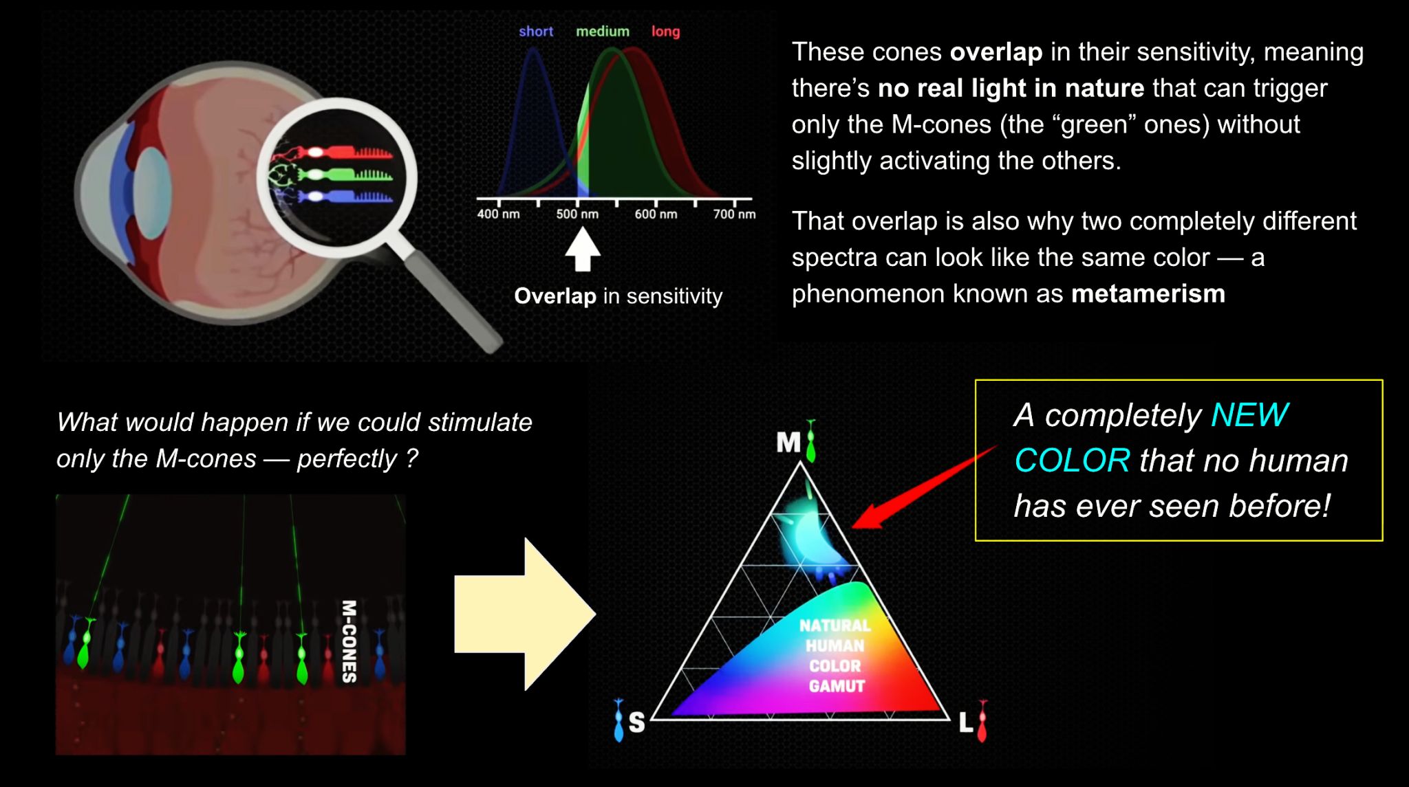
We introduce a principle, Oz, for displaying color imagery: directly controlling the human eye’s photoreceptor activity via cell-by-cell light delivery. Theoretically, novel colors are possible through bypassing the constraints set by the cone spectral sensitivities and activating M cone cells exclusively. In practice, we confirm a partial expansion of colorspace toward that theoretical ideal. Attempting to activate M cones exclusively is shown to elicit a color beyond the natural human gamut, formally measured with color matching by human subjects. They describe the color as blue-green of unprecedented saturation. Further experiments show that subjects perceive Oz colors in image and video form. The prototype targets laser microdoses to thousands of spectrally classified cones under fixational eye motion. These results are proof-of-principle for programmable control over individual photoreceptors at population scale.
A LUT (Lookup Table) is essentially the modifier between two images, the original image and the displayed image, based on a mathematical formula. Basically conversion matrices of different complexities. There are different types of LUTS – viewing, transform, calibration, 1D and 3D.
The cone angle of the sun refers to the angular diameter of the sun as observed from Earth, which is related to the apparent size of the sun in the sky.
The angular diameter of the sun, or the cone angle of the sunlight as perceived from Earth, is approximately 0.53 degrees on average. This value can vary slightly due to the elliptical nature of Earth’s orbit around the sun, but it generally stays within a narrow range.
Here’s a more precise breakdown:
Average Angular Diameter: About 0.53 degrees (31 arcminutes)
Minimum Angular Diameter: Approximately 0.52 degrees (when Earth is at aphelion, the farthest point from the sun)
Maximum Angular Diameter: Approximately 0.54 degrees (when Earth is at perihelion, the closest point to the sun)
This angular diameter remains relatively constant throughout the day because the sun’s distance from Earth does not change significantly over a single day.
To summarize, the cone angle of the sun’s light, or its angular diameter, is typically around 0.53 degrees, regardless of the time of day.
In general, when light interacts with matter, a complicated light-matter dynamic occurs. This interaction depends on the physical characteristics of the light as well as the physical composition and characteristics of the matter.
That is, some of the incident light is reflected, some of the light is transmitted, and another portion of the light is absorbed by the medium itself.
A BRDF describes how much light is reflected when light makes contact with a certain material. Similarly, a BTDF (Bi-directional Transmission Distribution Function) describes how much light is transmitted when light makes contact with a certain material
It is difficult to establish exactly how far one should go in elaborating the surface model. A truly complete representation of the reflective behavior of a surface might take into account such phenomena as polarization, scattering, fluorescence, and phosphorescence, all of which might vary with position on the surface. Therefore, the variables in this complete function would be:
incoming and outgoing angle incoming and outgoing wavelength incoming and outgoing polarization (both linear and circular) incoming and outgoing position (which might differ due to subsurface scattering) time delay between the incoming and outgoing light ray
RASTERIZATION Rasterisation (or rasterization) is the task of taking the information described in a vector graphics format OR the vertices of triangles making 3D shapes and converting them into a raster image (a series of pixels, dots or lines, which, when displayed together, create the image which was represented via shapes), or in other words “rasterizing” vectors or 3D models onto a 2D plane for display on a computer screen.
For each triangle of a 3D shape, you project the corners of the triangle on the virtual screen with some math (projective geometry). Then you have the position of the 3 corners of the triangle on the pixel screen. Those 3 points have texture coordinates, so you know where in the texture are the 3 corners. The cost is proportional to the number of triangles, and is only a little bit affected by the screen resolution.
In computer graphics, a raster graphics orbitmap image is a dot matrix data structure that represents a generally rectangular grid of pixels (points of color), viewable via a monitor, paper, or other display medium.
With rasterization, objects on the screen are created from a mesh of virtual triangles, or polygons, that create 3D models of objects. A lot of information is associated with each vertex, including its position in space, as well as information about color, texture and its “normal,” which is used to determine the way the surface of an object is facing.
Computers then convert the triangles of the 3D models into pixels, or dots, on a 2D screen. Each pixel can be assigned an initial color value from the data stored in the triangle vertices.
Further pixel processing or “shading,” including changing pixel color based on how lights in the scene hit the pixel, and applying one or more textures to the pixel, combine to generate the final color applied to a pixel.
The main advantage of rasterization is its speed. However, rasterization is simply the process of computing the mapping from scene geometry to pixels and does not prescribe a particular way to compute the color of those pixels. So it cannot take shading, especially the physical light, into account and it cannot promise to get a photorealistic output. That’s a big limitation of rasterization.
There are also multiple problems:
If you have two triangles one is behind the other, you will draw twice all the pixels. you only keep the pixel from the triangle that is closer to you (Z-buffer), but you still do the work twice.
The borders of your triangles are jagged as it is hard to know if a pixel is in the triangle or out. You can do some smoothing on those, that is anti-aliasing.
You have to handle every triangles (including the ones behind you) and then see that they do not touch the screen at all. (we have techniques to mitigate this where we only look at triangles that are in the field of view)
Transparency is hard to handle (you can’t just do an average of the color of overlapping transparent triangles, you have to do it in the right order)
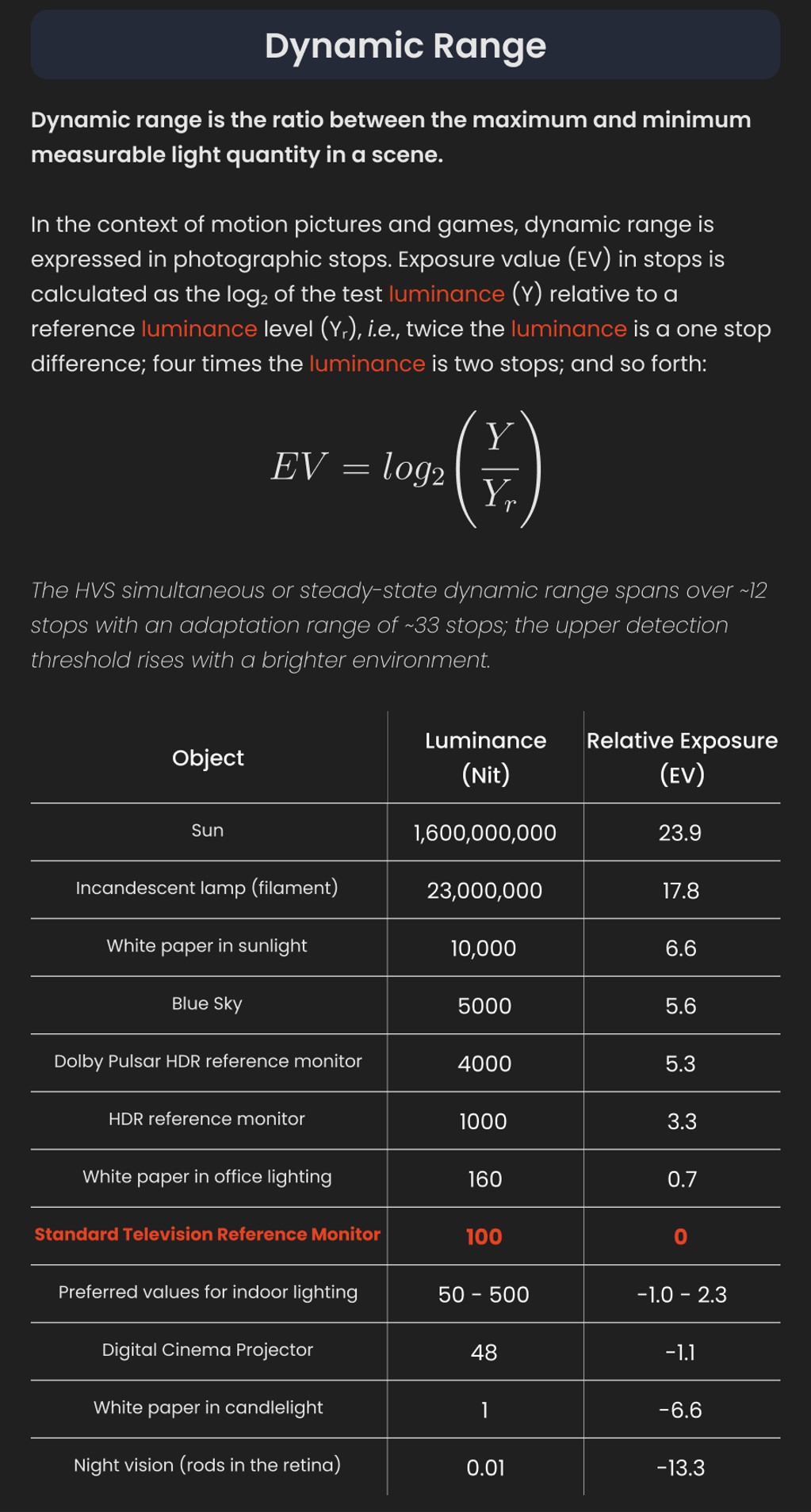
The dynamic range is a ratio between the maximum and minimum values of a physical measurement. Its definition depends on what the dynamic range refers to.
For a scene: Dynamic range is the ratio between the brightest and darkest parts of the scene.
For a camera: Dynamic range is the ratio of saturation to noise. More specifically, the ratio of the intensity that just saturates the camera to the intensity that just lifts the camera response one standard deviation above camera noise.
For a display: Dynamic range is the ratio between the maximum and minimum intensities emitted from the screen.
The Dynamic Range of real-world scenes can be quite high — ratios of 100,000:1 are common in the natural world. An HDR (High Dynamic Range) image stores pixel values that span the whole tonal range of real-world scenes. Therefore, an HDR image is encoded in a format that allows the largest range of values, e.g. floating-point values stored with 32 bits per color channel. Another characteristics of an HDR image is that it stores linear values. This means that the value of a pixel from an HDR image is proportional to the amount of light measured by the camera.
For TVs HDR is great, but it’s not the only new TV feature worth discussing.
This 2025 I decided to start learning how to code, so I installed Visual Studio and I started looking into C++. After days of watching tutorials and guides about the basics of C++ and programming, I decided to make something physics-related. I started with a dot that fell to the ground and then I wanted to simulate gravitational attraction, so I made 2 circles attracting each other. I thought it was really cool to see something I made with code actually work, so I kept building on top of that small, basic program. And here we are after roughly 8 months of learning programming. This is Galaxy Engine, and it is a simulation software I have been making ever since I started my learning journey. It currently can simulate gravity, dark matter, galaxies, the Big Bang, temperature, fluid dynamics, breakable solids, planetary interactions, etc. The program can run many tens of thousands of particles in real time on the CPU thanks to the Barnes-Hut algorithm, mixed with Morton curves. It also includes its own PBR 2D path tracer with BVH optimizations. The path tracer can simulate a bunch of stuff like diffuse lighting, specular reflections, refraction, internal reflection, fresnel, emission, dispersion, roughness, IOR, nested IOR and more! I tried to make the path tracer closer to traditional 3D render engines like V-Ray. I honestly never imagined I would go this far with programming, and it has been an amazing learning experience so far. I think that mixing this knowledge with my 3D knowledge can unlock countless new possibilities. In case you are curious about Galaxy Engine, I made it completely free and Open-Source so that anyone can build and compile it locally! You can find the source code inGitHub
DISCLAIMER – Links and images on this website may be protected by the respective owners’ copyright. All data submitted by users through this site shall be treated as freely available to share.