


COMPOSITION
-
StudioBinder – Roger Deakins on How to Choose a Camera Lens — Cinematography Composition Techniques
Read more: StudioBinder – Roger Deakins on How to Choose a Camera Lens — Cinematography Composition Techniques
https://www.studiobinder.com/blog/camera-lens-buying-guide/
https://www.studiobinder.com/blog/e-books/camera-lenses-explained-volume-1-ebook
-
Composition – These are the basic lighting techniques you need to know for photography and film
Read more: Composition – These are the basic lighting techniques you need to know for photography and film
http://www.diyphotography.net/basic-lighting-techniques-need-know-photography-film/
Amongst the basic techniques, there’s…
1- Side lighting – Literally how it sounds, lighting a subject from the side when they’re faced toward you
2- Rembrandt lighting – Here the light is at around 45 degrees over from the front of the subject, raised and pointing down at 45 degrees
3- Back lighting – Again, how it sounds, lighting a subject from behind. This can help to add drama with silouettes
4- Rim lighting – This produces a light glowing outline around your subject
5- Key light – The main light source, and it’s not necessarily always the brightest light source
6- Fill light – This is used to fill in the shadows and provide detail that would otherwise be blackness
7- Cross lighting – Using two lights placed opposite from each other to light two subjects


DESIGN


COLOR
-
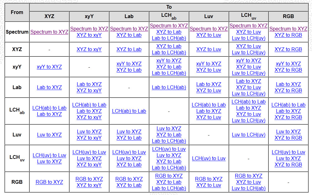
What is a Gamut or Color Space and why do I need to know about CIE
Read more: What is a Gamut or Color Space and why do I need to know about CIE

http://www.xdcam-user.com/2014/05/what-is-a-gamut-or-color-space-and-why-do-i-need-to-know-about-it/
In video terms gamut is normally related to as the full range of colours and brightness that can be either captured or displayed.
(more…) -
OLED vs QLED – What TV is better?
Read more: OLED vs QLED – What TV is better?
Supported by LG, Philips, Panasonic and Sony sell the OLED system TVs.
OLED stands for “organic light emitting diode.”
It is a fundamentally different technology from LCD, the major type of TV today.
OLED is “emissive,” meaning the pixels emit their own light.Samsung is branding its best TVs with a new acronym: “QLED”
QLED (according to Samsung) stands for “quantum dot LED TV.”
It is a variation of the common LED LCD, adding a quantum dot film to the LCD “sandwich.”
QLED, like LCD, is, in its current form, “transmissive” and relies on an LED backlight.OLED is the only technology capable of absolute blacks and extremely bright whites on a per-pixel basis. LCD definitely can’t do that, and even the vaunted, beloved, dearly departed plasma couldn’t do absolute blacks.
QLED, as an improvement over OLED, significantly improves the picture quality. QLED can produce an even wider range of colors than OLED, which says something about this new tech. QLED is also known to produce up to 40% higher luminance efficiency than OLED technology. Further, many tests conclude that QLED is far more efficient in terms of power consumption than its predecessor, OLED.
(more…) -
mmColorTarget – Nuke Gizmo for color matching a MacBeth chart
Read more: mmColorTarget – Nuke Gizmo for color matching a MacBeth charthttps://www.marcomeyer-vfx.de/posts/2014-04-11-mmcolortarget-nuke-gizmo/
https://www.marcomeyer-vfx.de/posts/mmcolortarget-nuke-gizmo/
https://vimeo.com/9.1652466e+07
https://www.nukepedia.com/gizmos/colour/mmcolortarget
-
Tobia Montanari – Memory Colors: an essential tool for Colorists
Read more: Tobia Montanari – Memory Colors: an essential tool for Coloristshttps://www.tobiamontanari.com/memory-colors-an-essential-tool-for-colorists/
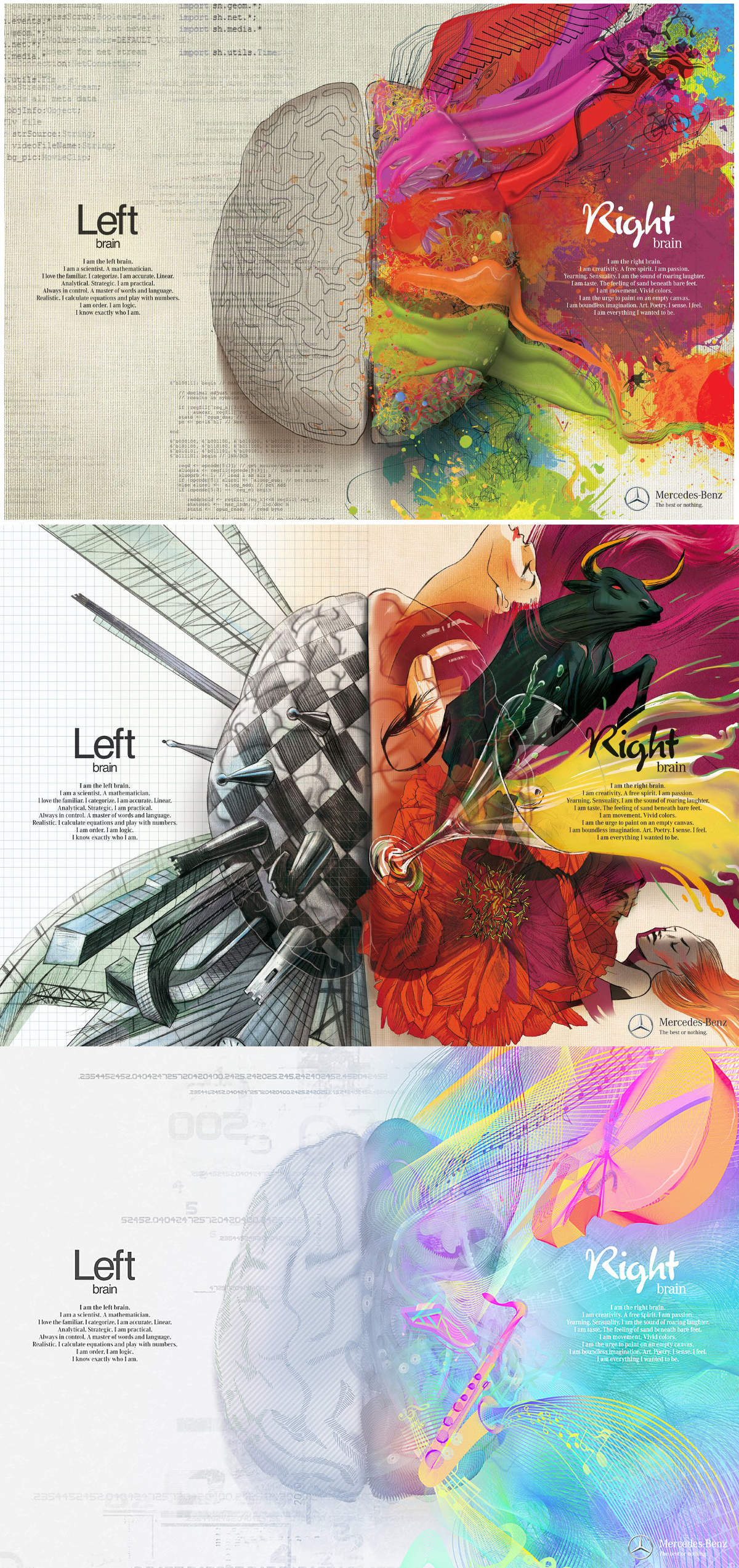
“Memory colors are colors that are universally associated with specific objects, elements or scenes in our environment. They are the colors that we expect to see in specific situations: these colors are based on our expectation of how certain objects should look based on our past experiences and memories.
For instance, we associate specific hues, saturation and brightness values with human skintones and a slight variation can significantly affect the way we perceive a scene.
Similarly, we expect blue skies to have a particular hue, green trees to be a specific shade and so on.
Memory colors live inside of our brains and we often impose them onto what we see. By considering them during the grading process, the resulting image will be more visually appealing and won’t distract the viewer from the intended message of the story. Even a slight deviation from memory colors in a movie can create a sense of discordance, ultimately detracting from the viewer’s experience.”


LIGHTING
-
Bella – Fast Spectral Rendering
Read more: Bella – Fast Spectral Rendering
Bella works in spectral space, allowing effects such as BSDF wavelength dependency, diffraction, or atmosphere to be modeled far more accurately than in color space.

https://superrendersfarm.com/blog/uncategorized/bella-a-new-spectral-physically-based-renderer/
-
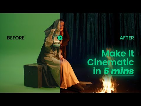
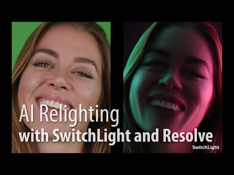
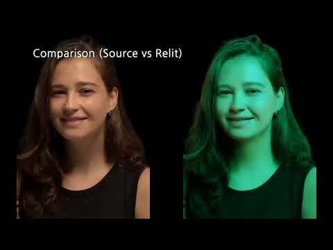
Beeble Switchlight’s Plugin for Foundry Nuke
Read more: Beeble Switchlight’s Plugin for Foundry Nukehttps://www.cutout.pro/learn/beeble-switchlight/
https://www.switchlight-api.beeble.ai/pricing
https://www.switchlight-api.beeble.ai
https://github.com/beeble-ai/SwitchLight-Studio
https://beeble.ai/terms-of-use
https://www.switchlight-api.beeble.ai/docs


-
Is a MacBeth Colour Rendition Chart the Safest Way to Calibrate a Camera?
Read more: Is a MacBeth Colour Rendition Chart the Safest Way to Calibrate a Camera?www.colour-science.org/posts/the-colorchecker-considered-mostly-harmless/
“Unless you have all the relevant spectral measurements, a colour rendition chart should not be used to perform colour-correction of camera imagery but only for white balancing and relative exposure adjustments.”
“Using a colour rendition chart for colour-correction might dramatically increase error if the scene light source spectrum is different from the illuminant used to compute the colour rendition chart’s reference values.”
“other factors make using a colour rendition chart unsuitable for camera calibration:
– Uncontrolled geometry of the colour rendition chart with the incident illumination and the camera.
– Unknown sample reflectances and ageing as the colour of the samples vary with time.
– Low samples count.
– Camera noise and flare.
– Etc…“Those issues are well understood in the VFX industry, and when receiving plates, we almost exclusively use colour rendition charts to white balance and perform relative exposure adjustments, i.e. plate neutralisation.”


COLLECTIONS
| Featured AI
| Design And Composition
| Explore posts
POPULAR SEARCHES
unreal | pipeline | virtual production | free | learn | photoshop | 360 | macro | google | nvidia | resolution | open source | hdri | real-time | photography basics | nuke
FEATURED POSTS
-
Photography basics: Solid Angle measures
-
Photography basics: Production Rendering Resolution Charts
-
The Public Domain Is Working Again — No Thanks To Disney
-
How to paint a boardgame miniatures
-
Types of Film Lights and their efficiency – CRI, Color Temperature and Luminous Efficacy
-
Top 3D Printing Website Resources
-
Matt Hallett – WAN 2.1 VACE Total Video Control in ComfyUI
-
Rec-2020 – TVs new color gamut standard used by Dolby Vision?
Social Links
DISCLAIMER – Links and images on this website may be protected by the respective owners’ copyright. All data submitted by users through this site shall be treated as freely available to share.
