


COMPOSITION
-
Composition – These are the basic lighting techniques you need to know for photography and film
Read more: Composition – These are the basic lighting techniques you need to know for photography and film
http://www.diyphotography.net/basic-lighting-techniques-need-know-photography-film/
Amongst the basic techniques, there’s…
1- Side lighting – Literally how it sounds, lighting a subject from the side when they’re faced toward you
2- Rembrandt lighting – Here the light is at around 45 degrees over from the front of the subject, raised and pointing down at 45 degrees
3- Back lighting – Again, how it sounds, lighting a subject from behind. This can help to add drama with silouettes
4- Rim lighting – This produces a light glowing outline around your subject
5- Key light – The main light source, and it’s not necessarily always the brightest light source
6- Fill light – This is used to fill in the shadows and provide detail that would otherwise be blackness
7- Cross lighting – Using two lights placed opposite from each other to light two subjects
-
Composition and The Expressive Nature Of Light
Read more: Composition and The Expressive Nature Of Lighthttp://www.huffingtonpost.com/bill-danskin/post_12457_b_10777222.html
George Sand once said “ The artist vocation is to send light into the human heart.”


DESIGN
-
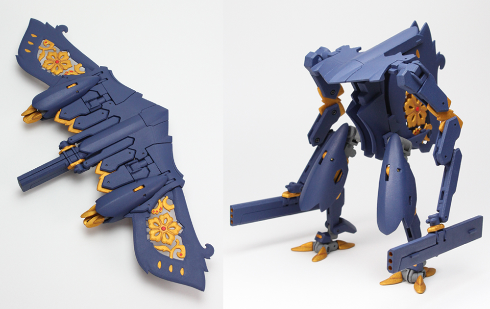
Japanese Designer Tomoo Yamaji Offers 3D Printed Transformer Kit, Stingray, Through Shapeways
Read more: Japanese Designer Tomoo Yamaji Offers 3D Printed Transformer Kit, Stingray, Through Shapewayshttps://3dprint.com/55799/transformer-kit-shapeways/
http://www.shapeways.com/product/5YHJL6XSZ/t060101-stingray?li=shareProduct


COLOR
-
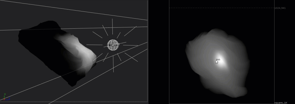
3D Lighting Tutorial by Amaan Kram
Read more: 3D Lighting Tutorial by Amaan Kramhttp://www.amaanakram.com/lightingT/part1.htm
The goals of lighting in 3D computer graphics are more or less the same as those of real world lighting.
Lighting serves a basic function of bringing out, or pushing back the shapes of objects visible from the camera’s view.
It gives a two-dimensional image on the monitor an illusion of the third dimension-depth.But it does not just stop there. It gives an image its personality, its character. A scene lit in different ways can give a feeling of happiness, of sorrow, of fear etc., and it can do so in dramatic or subtle ways. Along with personality and character, lighting fills a scene with emotion that is directly transmitted to the viewer.
Trying to simulate a real environment in an artificial one can be a daunting task. But even if you make your 3D rendering look absolutely photo-realistic, it doesn’t guarantee that the image carries enough emotion to elicit a “wow” from the people viewing it.
Making 3D renderings photo-realistic can be hard. Putting deep emotions in them can be even harder. However, if you plan out your lighting strategy for the mood and emotion that you want your rendering to express, you make the process easier for yourself.
Each light source can be broken down in to 4 distinct components and analyzed accordingly.
· Intensity
· Direction
· Color
· SizeThe overall thrust of this writing is to produce photo-realistic images by applying good lighting techniques.

-
The 7 key elements of brand identity design + 10 corporate identity examples
Read more: The 7 key elements of brand identity design + 10 corporate identity exampleswww.lucidpress.com/blog/the-7-key-elements-of-brand-identity-design
1. Clear brand purpose and positioning
2. Thorough market research
3. Likable brand personality
4. Memorable logo
5. Attractive color palette
6. Professional typography
7. On-brand supporting graphics

-
Photography basics: Why Use a (MacBeth) Color Chart?
Read more: Photography basics: Why Use a (MacBeth) Color Chart?Start here: https://www.pixelsham.com/2013/05/09/gretagmacbeth-color-checker-numeric-values/
https://www.studiobinder.com/blog/what-is-a-color-checker-tool/


In LightRoom

in Final Cut

in Nuke
Note: In Foundry’s Nuke, the software will map 18% gray to whatever your center f/stop is set to in the viewer settings (f/8 by default… change that to EV by following the instructions below).
You can experiment with this by attaching an Exposure node to a Constant set to 0.18, setting your viewer read-out to Spotmeter, and adjusting the stops in the node up and down. You will see that a full stop up or down will give you the respective next value on the aperture scale (f8, f11, f16 etc.).One stop doubles or halves the amount or light that hits the filmback/ccd, so everything works in powers of 2.
So starting with 0.18 in your constant, you will see that raising it by a stop will give you .36 as a floating point number (in linear space), while your f/stop will be f/11 and so on.If you set your center stop to 0 (see below) you will get a relative readout in EVs, where EV 0 again equals 18% constant gray.

In other words. Setting the center f-stop to 0 means that in a neutral plate, the middle gray in the macbeth chart will equal to exposure value 0. EV 0 corresponds to an exposure time of 1 sec and an aperture of f/1.0.
This will set the sun usually around EV12-17 and the sky EV1-4 , depending on cloud coverage.
To switch Foundry’s Nuke’s SpotMeter to return the EV of an image, click on the main viewport, and then press s, this opens the viewer’s properties. Now set the center f-stop to 0 in there. And the SpotMeter in the viewport will change from aperture and fstops to EV.
-
Thomas Mansencal – Colour Science for Python
Read more: Thomas Mansencal – Colour Science for Pythonhttps://thomasmansencal.substack.com/p/colour-science-for-python
https://www.colour-science.org/
Colour is an open-source Python package providing a comprehensive number of algorithms and datasets for colour science. It is freely available under the BSD-3-Clause terms.

-
Stefan Ringelschwandtner – LUT Inspector tool
Read more: Stefan Ringelschwandtner – LUT Inspector toolIt lets you load any .cube LUT right in your browser, see the RGB curves, and use a split view on the Granger Test Image to compare the original vs. LUT-applied version in real time — perfect for spotting hue shifts, saturation changes, and contrast tweaks.
https://mononodes.com/lut-inspector/


LIGHTING
-
IES Light Profiles and editing software
Read more: IES Light Profiles and editing softwarehttp://www.derekjenson.com/3d-blog/ies-light-profiles
https://ieslibrary.com/en/browse#ies
https://leomoon.com/store/shaders/ies-lights-pack
https://docs.arnoldrenderer.com/display/a5afmug/ai+photometric+light
IES profiles are useful for creating life-like lighting, as they can represent the physical distribution of light from any light source.
The IES format was created by the Illumination Engineering Society, and most lighting manufacturers provide IES profile for the lights they manufacture.


-
Types of Film Lights and their efficiency – CRI, Color Temperature and Luminous Efficacy
Read more: Types of Film Lights and their efficiency – CRI, Color Temperature and Luminous Efficacynofilmschool.com/types-of-film-lights
“Not every light performs the same way. Lights and lighting are tricky to handle. You have to plan for every circumstance. But the good news is, lighting can be adjusted. Let’s look at different factors that affect lighting in every scene you shoot. “
Use CRI, Luminous Efficacy and color temperature controls to match your needs.
Color Temperature
Color temperature describes the “color” of white light by a light source radiated by a perfect black body at a given temperature measured in degrees Kelvinhttps://www.pixelsham.com/2019/10/18/color-temperature/
CRI
“The Color Rendering Index is a measurement of how faithfully a light source reveals the colors of whatever it illuminates, it describes the ability of a light source to reveal the color of an object, as compared to the color a natural light source would provide. The highest possible CRI is 100. A CRI of 100 generally refers to a perfect black body, like a tungsten light source or the sun. “https://www.studiobinder.com/blog/what-is-color-rendering-index
(more…) -
About green screens
Read more: About green screenshackaday.com/2015/02/07/how-green-screen-worked-before-computers/
www.newtek.com/blog/tips/best-green-screen-materials/
www.chromawall.com/blog//chroma-key-green

Chroma Key Green, the color of green screens is also known as Chroma Green and is valued at approximately 354C in the Pantone color matching system (PMS).
Chroma Green can be broken down in many different ways. Here is green screen green as other values useful for both physical and digital production:
Green Screen as RGB Color Value: 0, 177, 64
Green Screen as CMYK Color Value: 81, 0, 92, 0
Green Screen as Hex Color Value: #00b140
Green Screen as Websafe Color Value: #009933Chroma Key Green is reasonably close to an 18% gray reflectance.
Illuminate your green screen with an uniform source with less than 2/3 EV variation.
The level of brightness at any given f-stop should be equivalent to a 90% white card under the same lighting. -
GretagMacbeth Color Checker Numeric Values and Middle Gray
Read more: GretagMacbeth Color Checker Numeric Values and Middle GrayThe human eye perceives half scene brightness not as the linear 50% of the present energy (linear nature values) but as 18% of the overall brightness. We are biased to perceive more information in the dark and contrast areas. A Macbeth chart helps with calibrating back into a photographic capture into this “human perspective” of the world.
https://en.wikipedia.org/wiki/Middle_gray
In photography, painting, and other visual arts, middle gray or middle grey is a tone that is perceptually about halfway between black and white on a lightness scale in photography and printing, it is typically defined as 18% reflectance in visible light

Light meters, cameras, and pictures are often calibrated using an 18% gray card[4][5][6] or a color reference card such as a ColorChecker. On the assumption that 18% is similar to the average reflectance of a scene, a grey card can be used to estimate the required exposure of the film.
https://en.wikipedia.org/wiki/ColorChecker
(more…)


COLLECTIONS
| Featured AI
| Design And Composition
| Explore posts
POPULAR SEARCHES
unreal | pipeline | virtual production | free | learn | photoshop | 360 | macro | google | nvidia | resolution | open source | hdri | real-time | photography basics | nuke
FEATURED POSTS
-
Photography basics: Shutter angle and shutter speed and motion blur
-
Top 3D Printing Website Resources
-
sRGB vs REC709 – An introduction and FFmpeg implementations
-
Convert 2D Images or Text to 3D Models
-
Survivorship Bias: The error resulting from systematically focusing on successes and ignoring failures. How a young statistician saved his planes during WW2.
-
MiniMax-Remover – Taming Bad Noise Helps Video Object Removal Rotoscoping
-
Advanced Computer Vision with Python OpenCV and Mediapipe
-
59 AI Filmmaking Tools For Your Workflow
Social Links
DISCLAIMER – Links and images on this website may be protected by the respective owners’ copyright. All data submitted by users through this site shall be treated as freely available to share.
