To measure the contrast ratio you will need a light meter. The process starts with you measuring the main source of light, or the key light.
Get a reading from the brightest area on the face of your subject. Then, measure the area lit by the secondary light, or fill light. To make sense of what you have just measured you have to understand that the information you have just gathered is in F-stops, a measure of light. With each additional F-stop, for example going one stop from f/1.4 to f/2.0, you create a doubling of light. The reverse is also true; moving one stop from f/8.0 to f/5.6 results in a halving of the light.
Since spending a lot of time recently with SDXL I’ve since made my way back to SD 1.5
While the models overall have less fidelity. There is just no comparing to the current motion models we have available for animatediff with 1.5 models.
To date this is one of my favorite pieces. Not because I think it’s even the best it can be. But because the workflow adjustments unlocked some very important ideas I can’t wait to try out.
Performance by @silkenkelly and @itxtheballerina on IG
Arminas created this using Juggernaut Xl model and QR Code Monster SDXL ControlNet.
His pipeline: Static Images – Forge UI. Upscaled with Leonardo AI universal upscaler. Animated with Runway ML and Minimax. Video upscale – Topaz Video AI. Composited in Adobe Premiere.
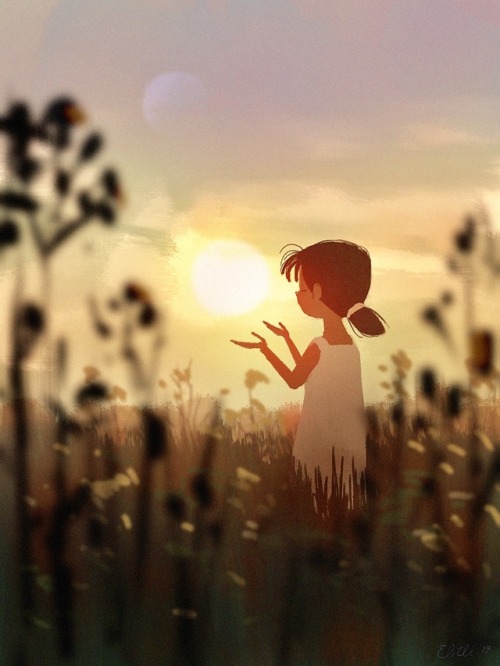
The way humans see the world… until we have a way to describe something, even something so fundamental as a colour, we may not even notice that something it’s there.
Ancient languages didn’t have a word for blue — not Greek, not Chinese, not Japanese, not Hebrew, not Icelandic cultures. And without a word for the colour, there’s evidence that they may not have seen it at all. https://www.wnycstudios.org/story/211119-colors
Every language first had a word for black and for white, or dark and light. The next word for a colour to come into existence — in every language studied around the world — was red, the colour of blood and wine. After red, historically, yellow appears, and later, green (though in a couple of languages, yellow and green switch places). The last of these colours to appear in every language is blue.
The only ancient culture to develop a word for blue was the Egyptians — and as it happens, they were also the only culture that had a way to produce a blue dye. https://mymodernmet.com/shades-of-blue-color-history/
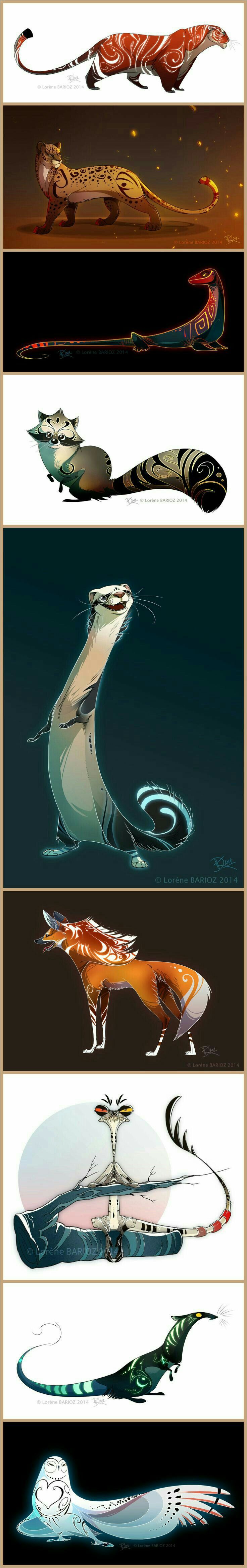
True blue hues are rare in the natural world because synthesizing pigments that absorb longer-wavelength light (reds and yellows) while reflecting shorter-wavelength blue light requires exceptionally elaborate molecular structures—biochemical feats that most plants and animals simply don’t undertake.
When you gaze at a blueberry’s deep blue surface, you’re actually seeing structural coloration rather than a true blue pigment. A fine, waxy bloom on the berry’s skin contains nanostructures that preferentially scatter blue and violet light, giving the fruit its signature blue sheen even though its inherent pigment is reddish.
Similarly, many of nature’s most striking blues—like those of blue jays and morpho butterflies—arise not from blue pigments but from microscopic architectures in feathers or wing scales. These tiny ridges and air pockets manipulate incoming light so that blue wavelengths emerge most prominently, creating vivid, angle-dependent colors through scattering rather than pigment alone.
This help’s us understand the composition of components in/on solar system bodies.
Dips in the observed light spectrum, also known as, lines of absorption occur as gasses absorb energy from light at specific points along the light spectrum.
These dips or darkened zones (lines of absorption) leave a finger print which identify elements and compounds.
In this image the dark absorption bands appear as lines of emission which occur as the result of emitted not reflected (absorbed) light.
The Manuka rendering architecture has been designed in the spirit of the classic reyes rendering architecture. In its core, reyes is based on stochastic rasterisation of micropolygons, facilitating depth of field, motion blur, high geometric complexity,and programmable shading.
This is commonly achieved with Monte Carlo path tracing, using a paradigm often called shade-on-hit, in which the renderer alternates tracing rays with running shaders on the various ray hits. The shaders take the role of generating the inputs of the local material structure which is then used bypath sampling logic to evaluate contributions and to inform what further rays to cast through the scene.
Over the years, however, the expectations have risen substantially when it comes to image quality. Computing pictures which are indistinguishable from real footage requires accurate simulation of light transport, which is most often performed using some variant of Monte Carlo path tracing. Unfortunately this paradigm requires random memory accesses to the whole scene and does not lend itself well to a rasterisation approach at all.
Manuka is both a uni-directional and bidirectional path tracer and encompasses multiple importance sampling (MIS). Interestingly, and importantly for production character skin work, it is the first major production renderer to incorporate spectral MIS in the form of a new ‘Hero Spectral Sampling’ technique, which was recently published at Eurographics Symposium on Rendering 2014.
Manuka propose a shade-before-hit paradigm in-stead and minimise I/O strain (and some memory costs) on the system, leveraging locality of reference by running pattern generation shaders before we execute light transport simulation by path sampling, “compressing” any bvh structure as needed, and as such also limiting duplication of source data.
The difference with reyes is that instead of baking colors into the geometry like in Reyes, manuka bakes surface closures. This means that light transport is still calculated with path tracing, but all texture lookups etc. are done up-front and baked into the geometry.
The main drawback with this method is that geometry has to be tessellated to its highest, stable topology before shading can be evaluated properly. As such, the high cost to first pixel. Even a basic 4 vertices square becomes a much more complex model with this approach.
Manuka use the RenderMan Shading Language (rsl) for programmable shading [Pixar Animation Studios 2015], but we do not invoke rsl shaders when intersecting a ray with a surface (often called shade-on-hit). Instead, we pre-tessellate and pre-shade all the input geometry in the front end of the renderer.
This way, we can efficiently order shading computations to sup-port near-optimal texture locality, vectorisation, and parallelism. This system avoids repeated evaluation of shaders at the same surface point, and presents a minimal amount of memory to be accessed during light transport time. An added benefit is that the acceleration structure for ray tracing (abounding volume hierarchy, bvh) is built once on the final tessellated geometry, which allows us to ray trace more efficiently than multi-level bvhs and avoids costly caching of on-demand tessellated micropolygons and the associated scheduling issues.
For the shading reasons above, in terms of AOVs, the studio approach is to succeed at combining complex shading with ray paths in the render rather than pass a multi-pass render to compositing.
For the Spectral Rendering component. The light transport stage is fully spectral, using a continuously sampled wavelength which is traced with each path and used to apply the spectral camera sensitivity of the sensor. This allows for faithfully support any degree of observer metamerism as the camera footage they are intended to match as well as complex materials which require wavelength dependent phenomena such as diffraction, dispersion, interference, iridescence, or chromatic extinction and Rayleigh scattering in participating media.
As opposed to the original reyes paper, we use bilinear interpolation of these bsdf inputs later when evaluating bsdfs per pathv ertex during light transport4. This improves temporal stability of geometry which moves very slowly with respect to the pixel raster
In terms of the pipeline, everything rendered at Weta was already completely interwoven with their deep data pipeline. Manuka very much was written with deep data in mind. Here, Manuka not so much extends the deep capabilities, rather it fully matches the already extremely complex and powerful setup Weta Digital already enjoy with RenderMan. For example, an ape in a scene can be selected, its ID is available and a NUKE artist can then paint in 3D say a hand and part of the way up the neutral posed ape.
We called our system Manuka, as a respectful nod to reyes: we had heard a story froma former ILM employee about how reyes got its name from how fond the early Pixar people were of their lunches at Point Reyes, and decided to name our system after our surrounding natural environment, too. Manuka is a kind of tea tree very common in New Zealand which has very many very small leaves, in analogy to micropolygons ina tree structure for ray tracing. It also happens to be the case that Weta Digital’s main site is on Manuka Street.
Note: In Foundry’s Nuke, the software will map 18% gray to whatever your center f/stop is set to in the viewer settings (f/8 by default… change that to EV by following the instructions below).
You can experiment with this by attaching an Exposure node to a Constant set to 0.18, setting your viewer read-out to Spotmeter, and adjusting the stops in the node up and down. You will see that a full stop up or down will give you the respective next value on the aperture scale (f8, f11, f16 etc.).
One stop doubles or halves the amount or light that hits the filmback/ccd, so everything works in powers of 2.
So starting with 0.18 in your constant, you will see that raising it by a stop will give you .36 as a floating point number (in linear space), while your f/stop will be f/11 and so on.
If you set your center stop to 0 (see below) you will get a relative readout in EVs, where EV 0 again equals 18% constant gray.
In other words. Setting the center f-stop to 0 means that in a neutral plate, the middle gray in the macbeth chart will equal to exposure value 0. EV 0 corresponds to an exposure time of 1 sec and an aperture of f/1.0.
This will set the sun usually around EV12-17 and the sky EV1-4 , depending on cloud coverage.
To switch Foundry’s Nuke’s SpotMeter to return the EV of an image, click on the main viewport, and then press s, this opens the viewer’s properties. Now set the center f-stop to 0 in there. And the SpotMeter in the viewport will change from aperture and fstops to EV.
A measure of how large the object appears to an observer looking from that point. Thus. A measure for objects in the sky. Useful to retuen the size of the sun and moon… and in perspective, how much of their contribution to lighting. Solid angle can be represented in ‘angular diameter’ as well.
A solid angle is expressed in a dimensionless unit called a steradian (symbol: sr). By default in terms of the total celestial sphere and before atmospheric’s scattering, the Sun and the Moon subtend fractional areas of 0.000546% (Sun) and 0.000531% (Moon).
On earth the sun is likely closer to 0.00011 solid angle after athmospheric scattering. The sun as perceived from earth has a diameter of 0.53 degrees. This is about 0.000064 solid angle.
The mean angular diameter of the full moon is 2q = 0.52° (it varies with time around that average, by about 0.009°). This translates into a solid angle of 0.0000647 sr, which means that the whole night sky covers a solid angle roughly one hundred thousand times greater than the full moon.
The apparent size of an object as seen by an observer; expressed in units of degrees (of arc), arc minutes, or arc seconds. The moon, as viewed from the Earth, has an angular diameter of one-half a degree.
The angle covered by the diameter of the full moon is about 31 arcmin or 1/2°, so astronomers would say the Moon’s angular diameter is 31 arcmin, or the Moon subtends an angle of 31 arcmin.
In general, when light interacts with matter, a complicated light-matter dynamic occurs. This interaction depends on the physical characteristics of the light as well as the physical composition and characteristics of the matter.
That is, some of the incident light is reflected, some of the light is transmitted, and another portion of the light is absorbed by the medium itself.
A BRDF describes how much light is reflected when light makes contact with a certain material. Similarly, a BTDF (Bi-directional Transmission Distribution Function) describes how much light is transmitted when light makes contact with a certain material
It is difficult to establish exactly how far one should go in elaborating the surface model. A truly complete representation of the reflective behavior of a surface might take into account such phenomena as polarization, scattering, fluorescence, and phosphorescence, all of which might vary with position on the surface. Therefore, the variables in this complete function would be:
incoming and outgoing angle incoming and outgoing wavelength incoming and outgoing polarization (both linear and circular) incoming and outgoing position (which might differ due to subsurface scattering) time delay between the incoming and outgoing light ray
DISCLAIMER – Links and images on this website may be protected by the respective owners’ copyright. All data submitted by users through this site shall be treated as freely available to share.


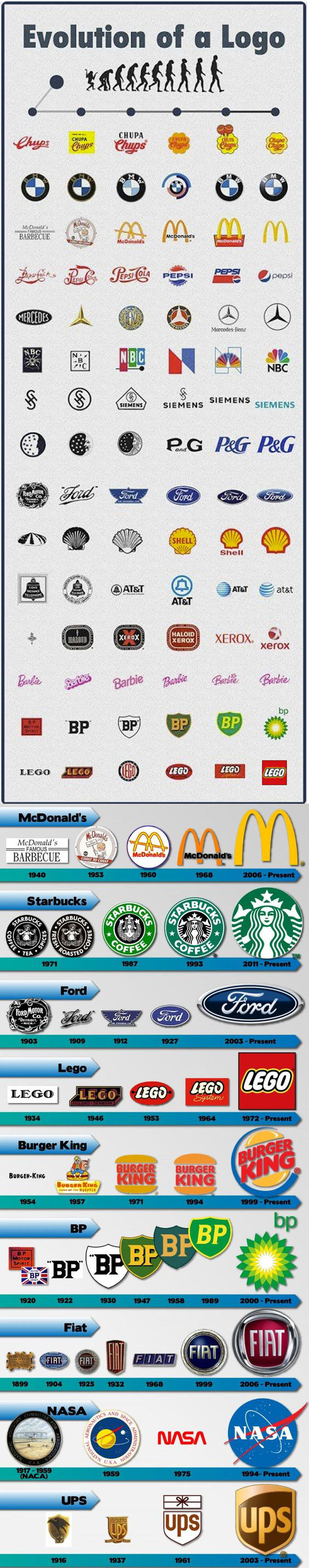


 Lines of emission