Depth of field is the range within which focusing is resolved in a photo.
Aperture has a huge affect on to the depth of field.
Changing the f-stops (f/#) of a lens will change aperture and as such the DOF.
f-stops are a just certain number which is telling you the size of the aperture. That’s how f-stop is related to aperture (and DOF).
If you increase f-stops, it will increase DOF, the area in focus (and decrease the aperture). On the other hand, decreasing the f-stop it will decrease DOF (and increase the aperture).
The red cone in the figure is an angular representation of the resolution of the system. Versus the dotted lines, which indicate the aperture coverage. Where the lines of the two cones intersect defines the total range of the depth of field.
This image explains why the longer the depth of field, the greater the range of clarity.
1. Watch every frame of raw footage twice. On the second time, take notes. If you don’t do this and try to start developing a scene premature, then it’s a big disservice to yourself and to the director, actors and production crew.
2. Nurture the relationships with the director. You are the secondary person in the relationship. Be calm and continually offer solutions. Get the main intention of the film as soon as possible from the director.
3. Organize your media so that you can find any shot instantly.
4. Factor in extra time for renders, exports, errors and crashes.
5. Attempt edits and ideas that shouldn’t work. It just might work. Until you do it and watch it, you won’t know. Don’t rule out ideas just because they don’t make sense in your mind.
6. Spend more time on your audio. It’s the glue of your edit. AUDIO SAVES EVERYTHING. Create fluid and seamless audio under your video.
7. Make cuts for the scene, but always in context for the whole film. Have a macro and a micro view at all times.
To measure the contrast ratio you will need a light meter. The process starts with you measuring the main source of light, or the key light.
Get a reading from the brightest area on the face of your subject. Then, measure the area lit by the secondary light, or fill light. To make sense of what you have just measured you have to understand that the information you have just gathered is in F-stops, a measure of light. With each additional F-stop, for example going one stop from f/1.4 to f/2.0, you create a doubling of light. The reverse is also true; moving one stop from f/8.0 to f/5.6 results in a halving of the light.
“Not every light performs the same way. Lights and lighting are tricky to handle. You have to plan for every circumstance. But the good news is, lighting can be adjusted. Let’s look at different factors that affect lighting in every scene you shoot. “
Use CRI, Luminous Efficacy and color temperature controls to match your needs.
Color Temperature Color temperature describes the “color” of white light by a light source radiated by a perfect black body at a given temperature measured in degrees Kelvin
CRI “The Color Rendering Index is a measurement of how faithfully a light source reveals the colors of whatever it illuminates, it describes the ability of a light source to reveal the color of an object, as compared to the color a natural light source would provide. The highest possible CRI is 100. A CRI of 100 generally refers to a perfect black body, like a tungsten light source or the sun. “
Spectralon is a teflon-based pressed powderthat comes closest to being a pure Lambertian diffuse material that reflects 100% of all light. If we take an HDR photograph of the Spectralon alongside the material to be measured, we can derive thediffuse albedo of that material.
The process to capture diffuse reflectance is very similar to the one outlined by Hable.
1. We put a linear polarizing filter in front of the camera lens and a second linear polarizing filterin front of a modeling light or a flash such that the two filters are oriented perpendicular to eachother, i.e. cross polarized.
2. We place Spectralon close to and parallel with the material we are capturing and take brack-eted shots of the setup7. Typically, we’ll take nine photographs, from -4EV to +4EV in 1EVincrements.
3. We convert the bracketed shots to a linear HDR image. We found that many HDR packagesdo not produce an HDR image in which the pixel values are linear. PTGui is an example of apackage which does generate a linear HDR image. At this point, because of the cross polarization,the image is one of surface diffuse response.
4. We open the file in Photoshop and normalize the image by color picking the Spectralon, filling anew layer with that color and setting that layer to “Divide”. This sets the Spectralon to 1 in theimage. All other color values are relative to this so we can consider them as diffuse albedo.
A light wave that is vibrating in more than one plane is referred to as unpolarized light. …
Polarized light waves are light waves in which the vibrations occur in a single plane. The process of transforming unpolarized light into polarized light is known as polarization.
The most common use of polarized technology is to reduce lighting complexity on the subject. Details such as glare and hard edges are not removed, but greatly reduced.
Most software around us today are decent at accurately displaying colors. Processing of colors is another story unfortunately, and is often done badly.
To understand what the problem is, let’s start with an example of three ways of blending green and magenta:
Perceptual blend – A smooth transition using a model designed to mimic human perception of color. The blending is done so that the perceived brightness and color varies smoothly and evenly.
Linear blend – A model for blending color based on how light behaves physically. This type of blending can occur in many ways naturally, for example when colors are blended together by focus blur in a camera or when viewing a pattern of two colors at a distance.
sRGB blend – This is how colors would normally be blended in computer software, using sRGB to represent the colors.
Let’s look at some more examples of blending of colors, to see how these problems surface more practically. The examples use strong colors since then the differences are more pronounced. This is using the same three ways of blending colors as the first example.
Instead of making it as easy as possible to work with color, most software make it unnecessarily hard, by doing image processing with representations not designed for it. Approximating the physical behavior of light with linear RGB models is one easy thing to do, but more work is needed to create image representations tailored for image processing and human perception.
This page compares images rendered in Arnold using spectral rendering and different sets of colourspace primaries: Rec.709, Rec.2020, ACES and DCI-P3. The SPD data for the GretagMacbeth Color Checker are the measurements of Noburu Ohta, taken from Mansencal, Mauderer and Parsons (2014) colour-science.org.
A measure of how large the object appears to an observer looking from that point. Thus. A measure for objects in the sky. Useful to retuen the size of the sun and moon… and in perspective, how much of their contribution to lighting. Solid angle can be represented in ‘angular diameter’ as well.
A solid angle is expressed in a dimensionless unit called a steradian (symbol: sr). By default in terms of the total celestial sphere and before atmospheric’s scattering, the Sun and the Moon subtend fractional areas of 0.000546% (Sun) and 0.000531% (Moon).
On earth the sun is likely closer to 0.00011 solid angle after athmospheric scattering. The sun as perceived from earth has a diameter of 0.53 degrees. This is about 0.000064 solid angle.
The mean angular diameter of the full moon is 2q = 0.52° (it varies with time around that average, by about 0.009°). This translates into a solid angle of 0.0000647 sr, which means that the whole night sky covers a solid angle roughly one hundred thousand times greater than the full moon.
The apparent size of an object as seen by an observer; expressed in units of degrees (of arc), arc minutes, or arc seconds. The moon, as viewed from the Earth, has an angular diameter of one-half a degree.
The angle covered by the diameter of the full moon is about 31 arcmin or 1/2°, so astronomers would say the Moon’s angular diameter is 31 arcmin, or the Moon subtends an angle of 31 arcmin.
Physically-based shading means leaving behind phenomenological models, like the Phong shading model, which are simply built to “look good” subjectively without being based on physics in any real way, and moving to lighting and shading models that are derived from the laws of physics and/or from actual measurements of the real world, and rigorously obey physical constraints such as energy conservation.
For example, in many older rendering systems, shading models included separate controls for specular highlights from point lights and reflection of the environment via a cubemap. You could create a shader with the specular and the reflection set to wildly different values, even though those are both instances of the same physical process. In addition, you could set the specular to any arbitrary brightness, even if it would cause the surface to reflect more energy than it actually received.
In a physically-based system, both the point light specular and the environment reflection would be controlled by the same parameter, and the system would be set up to automatically adjust the brightness of both the specular and diffuse components to maintain overall energy conservation. Moreover you would want to set the specular brightness to a realistic value for the material you’re trying to simulate, based on measurements.
Physically-based lighting or shading includes physically-based BRDFs, which are usually based on microfacet theory, and physically correct light transport, which is based on the rendering equation (although heavily approximated in the case of real-time games).
It also includes the necessary changes in the art process to make use of these features. Switching to a physically-based system can cause some upsets for artists. First of all it requires full HDR lighting with a realistic level of brightness for light sources, the sky, etc. and this can take some getting used to for the lighting artists. It also requires texture/material artists to do some things differently (particularly for specular), and they can be frustrated by the apparent loss of control (e.g. locking together the specular highlight and environment reflection as mentioned above; artists will complain about this). They will need some time and guidance to adapt to the physically-based system.
On the plus side, once artists have adapted and gained trust in the physically-based system, they usually end up liking it better, because there are fewer parameters overall (less work for them to tweak). Also, materials created in one lighting environment generally look fine in other lighting environments too. This is unlike more ad-hoc models, where a set of material parameters might look good during daytime, but it comes out ridiculously glowy at night, or something like that.
Here are some resources to look at for physically-based lighting in games:
SIGGRAPH 2013 Physically Based Shading Course, particularly the background talk by Naty Hoffman at the beginning. You can also check out the previous incarnations of this course for more resources.
And of course, I would be remiss if I didn’t mention Physically-Based Rendering by Pharr and Humphreys, an amazing reference on this whole subject and well worth your time, although it focuses on offline rather than real-time rendering.
Bella works in spectral space, allowing effects such as BSDF wavelength dependency, diffraction, or atmosphere to be modeled far more accurately than in color space.
A way to approximate complex lighting in ultra realistic renders.
All SH lighting techniques involve replacing parts of standard lighting equations with spherical functions that have been projected into frequency space using the spherical harmonics as a basis.
Size. Mr. White (Harvey Keitel) on the right. Focus. He’s one of the two objects in focus. Lighting. Mr. White is large and in focus and Mr. Pink (Steve Buscemi) is highlighted by a shaft of light. Color. Both are black and white but the read on Mr. White’s shirt now really stands out.
DISCLAIMER – Links and images on this website may be protected by the respective owners’ copyright. All data submitted by users through this site shall be treated as freely available to share.