


COMPOSITION
-
Photography basics: Depth of Field and composition
Read more: Photography basics: Depth of Field and compositionDepth of field is the range within which focusing is resolved in a photo.
Aperture has a huge affect on to the depth of field.
Changing the f-stops (f/#) of a lens will change aperture and as such the DOF.
f-stops are a just certain number which is telling you the size of the aperture. That’s how f-stop is related to aperture (and DOF).
If you increase f-stops, it will increase DOF, the area in focus (and decrease the aperture). On the other hand, decreasing the f-stop it will decrease DOF (and increase the aperture).
The red cone in the figure is an angular representation of the resolution of the system. Versus the dotted lines, which indicate the aperture coverage. Where the lines of the two cones intersect defines the total range of the depth of field.
This image explains why the longer the depth of field, the greater the range of clarity.

-
7 Commandments of Film Editing and composition
Read more: 7 Commandments of Film Editing and composition
1. Watch every frame of raw footage twice. On the second time, take notes. If you don’t do this and try to start developing a scene premature, then it’s a big disservice to yourself and to the director, actors and production crew.
2. Nurture the relationships with the director. You are the secondary person in the relationship. Be calm and continually offer solutions. Get the main intention of the film as soon as possible from the director.
3. Organize your media so that you can find any shot instantly.
4. Factor in extra time for renders, exports, errors and crashes.
5. Attempt edits and ideas that shouldn’t work. It just might work. Until you do it and watch it, you won’t know. Don’t rule out ideas just because they don’t make sense in your mind.
6. Spend more time on your audio. It’s the glue of your edit. AUDIO SAVES EVERYTHING. Create fluid and seamless audio under your video.
7. Make cuts for the scene, but always in context for the whole film. Have a macro and a micro view at all times.


DESIGN


COLOR
-
The 7 key elements of brand identity design + 10 corporate identity examples
Read more: The 7 key elements of brand identity design + 10 corporate identity exampleswww.lucidpress.com/blog/the-7-key-elements-of-brand-identity-design
1. Clear brand purpose and positioning
2. Thorough market research
3. Likable brand personality
4. Memorable logo
5. Attractive color palette
6. Professional typography
7. On-brand supporting graphics

-
Victor Perez – The Color Management Handbook for Visual Effects Artists
Read more: Victor Perez – The Color Management Handbook for Visual Effects ArtistsDigital Color Principles, Color Management Fundamentals & ACES Workflows

-
Practical Aspects of Spectral Data and LEDs in Digital Content Production and Virtual Production – SIGGRAPH 2022
Read more: Practical Aspects of Spectral Data and LEDs in Digital Content Production and Virtual Production – SIGGRAPH 2022
Comparison to the commercial side

https://www.ecolorled.com/blog/detail/what-is-rgb-rgbw-rgbic-strip-lights
RGBW (RGB + White) LED strip uses a 4-in-1 LED chip made up of red, green, blue, and white.
RGBWW (RGB + White + Warm White) LED strip uses either a 5-in-1 LED chip with red, green, blue, white, and warm white for color mixing. The only difference between RGBW and RGBWW is the intensity of the white color. The term RGBCCT consists of RGB and CCT. CCT (Correlated Color Temperature) means that the color temperature of the led strip light can be adjusted to change between warm white and white. Thus, RGBWW strip light is another name of RGBCCT strip.
RGBCW is the acronym for Red, Green, Blue, Cold, and Warm. These 5-in-1 chips are used in supper bright smart LED lighting products
-
“Reality” is constructed by your brain. Here’s what that means, and why it matters.
Read more: “Reality” is constructed by your brain. Here’s what that means, and why it matters.“Fix your gaze on the black dot on the left side of this image. But wait! Finish reading this paragraph first. As you gaze at the left dot, try to answer this question: In what direction is the object on the right moving? Is it drifting diagonally, or is it moving up and down?”

What color are these strawberries?

Are A and B the same gray?

-
The Maya civilization and the color blue
Read more: The Maya civilization and the color blueMaya blue is a highly unusual pigment because it is a mix of organic indigo and an inorganic clay mineral called palygorskite.
Echoing the color of an azure sky, the indelible pigment was used to accentuate everything from ceramics to human sacrifices in the Late Preclassic period (300 B.C. to A.D. 300).
A team of researchers led by Dean Arnold, an adjunct curator of anthropology at the Field Museum in Chicago, determined that the key to Maya blue was actually a sacred incense called copal.
By heating the mixture of indigo, copal and palygorskite over a fire, the Maya produced the unique pigment, he reported at the time.
-
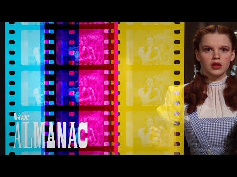
Scientists claim to have discovered ‘new colour’ no one has seen before: Olo
Read more: Scientists claim to have discovered ‘new colour’ no one has seen before: Olohttps://www.bbc.com/news/articles/clyq0n3em41o
By stimulating specific cells in the retina, the participants claim to have witnessed a blue-green colour that scientists have called “olo”, but some experts have said the existence of a new colour is “open to argument”.
The findings, published in the journal Science Advances on Friday, have been described by the study’s co-author, Prof Ren Ng from the University of California, as “remarkable”.

(A) System inputs. (i) Retina map of 103 cone cells preclassified by spectral type (7). (ii) Target visual percept (here, a video of a child, see movie S1 at 1:04). (iii) Infrared cellular-scale imaging of the retina with 60-frames-per-second rolling shutter. Fixational eye movement is visible over the three frames shown.
(B) System outputs. (iv) Real-time per-cone target activation levels to reproduce the target percept, computed by: extracting eye motion from the input video relative to the retina map; identifying the spectral type of every cone in the field of view; computing the per-cone activation the target percept would have produced. (v) Intensities of visible-wavelength 488-nm laser microdoses at each cone required to achieve its target activation level.
(C) Infrared imaging and visible-wavelength stimulation are physically accomplished in a raster scan across the retinal region using AOSLO. By modulating the visible-wavelength beam’s intensity, the laser microdoses shown in (v) are delivered. Drawing adapted with permission [Harmening and Sincich (54)].
(D) Examples of target percepts with corresponding cone activations and laser microdoses, ranging from colored squares to complex imagery. Teal-striped regions represent the color “olo” of stimulating only M cones.
-
RawTherapee – a free, open source, cross-platform raw image and HDRi processing program
Read more: RawTherapee – a free, open source, cross-platform raw image and HDRi processing program5.10 of this tool includes excellent tools to clean up cr2 and cr3 used on set to support HDRI processing.
Converting raw to AcesCG 32 bit tiffs with metadata.


LIGHTING
-
Lighting Every Darkness with 3DGS: Fast Training and Real-Time Rendering and Denoising for HDR View Synthesis
Read more: Lighting Every Darkness with 3DGS: Fast Training and Real-Time Rendering and Denoising for HDR View Synthesishttps://srameo.github.io/projects/le3d/
LE3D is a method for real-time HDR view synthesis from RAW images. It is particularly effective for nighttime scenes.
https://github.com/Srameo/LE3D


-
Terminators and Iron Men: HDRI, Image-based lighting and physical shading at ILM – Siggraph 2010
Read more: Terminators and Iron Men: HDRI, Image-based lighting and physical shading at ILM – Siggraph 2010 -
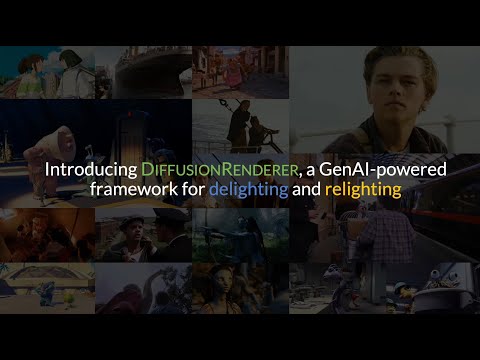
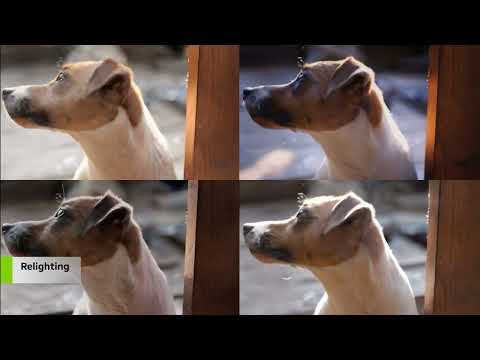
NVidia DiffusionRenderer – Neural Inverse and Forward Rendering with Video Diffusion Models. How NVIDIA reimagined relighting
Read more: NVidia DiffusionRenderer – Neural Inverse and Forward Rendering with Video Diffusion Models. How NVIDIA reimagined relightinghttps://www.fxguide.com/quicktakes/diffusing-reality-how-nvidia-reimagined-relighting/
https://research.nvidia.com/labs/toronto-ai/DiffusionRenderer/
-
Photography basics: Color Temperature and White Balance
Read more: Photography basics: Color Temperature and White Balance

Color Temperature of a light source describes the spectrum of light which is radiated from a theoretical “blackbody” (an ideal physical body that absorbs all radiation and incident light – neither reflecting it nor allowing it to pass through) with a given surface temperature.
https://en.wikipedia.org/wiki/Color_temperature
Or. Most simply it is a method of describing the color characteristics of light through a numerical value that corresponds to the color emitted by a light source, measured in degrees of Kelvin (K) on a scale from 1,000 to 10,000.
More accurately. The color temperature of a light source is the temperature of an ideal backbody that radiates light of comparable hue to that of the light source.
(more…)


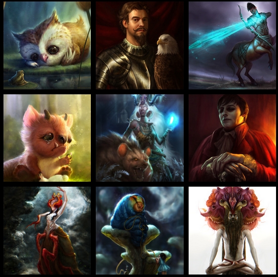
COLLECTIONS
| Featured AI
| Design And Composition
| Explore posts
POPULAR SEARCHES
unreal | pipeline | virtual production | free | learn | photoshop | 360 | macro | google | nvidia | resolution | open source | hdri | real-time | photography basics | nuke
FEATURED POSTS
-
AnimationXpress.com interviews Daniele Tosti for TheCgCareer.com channel
-
Survivorship Bias: The error resulting from systematically focusing on successes and ignoring failures. How a young statistician saved his planes during WW2.
-
Embedding frame ranges into Quicktime movies with FFmpeg
-
3D Gaussian Splatting step by step beginner course
-
WhatDreamsCost Spline-Path-Control – Create motion controls for ComfyUI
-
Generative AI Glossary / AI Dictionary / AI Terminology
-
Ethan Roffler interviews CG Supervisor Daniele Tosti
-
HDRI Median Cut plugin
Social Links
DISCLAIMER – Links and images on this website may be protected by the respective owners’ copyright. All data submitted by users through this site shall be treated as freely available to share.
