“Not every light performs the same way. Lights and lighting are tricky to handle. You have to plan for every circumstance. But the good news is, lighting can be adjusted. Let’s look at different factors that affect lighting in every scene you shoot. “
Use CRI, Luminous Efficacy and color temperature controls to match your needs.
Color Temperature Color temperature describes the “color” of white light by a light source radiated by a perfect black body at a given temperature measured in degrees Kelvin
CRI “The Color Rendering Index is a measurement of how faithfully a light source reveals the colors of whatever it illuminates, it describes the ability of a light source to reveal the color of an object, as compared to the color a natural light source would provide. The highest possible CRI is 100. A CRI of 100 generally refers to a perfect black body, like a tungsten light source or the sun. “
The intricate relationship between the eyes and the brain, often termed the eye-mind connection, reveals that vision is predominantly a cognitive process. This understanding has profound implications for fields such as design, where capturing and maintaining attention is paramount. This essay delves into the nuances of visual perception, the brain’s role in interpreting visual data, and how this knowledge can be applied to effective design strategies.
This cognitive aspect of vision is evident in phenomena such as optical illusions, where the brain interprets visual information in a way that contradicts physical reality. These illusions underscore that what we “see” is not merely a direct recording of the external world but a constructed experience shaped by cognitive processes.
Understanding the cognitive nature of vision is crucial for effective design. Designers must consider how the brain processes visual information to create compelling and engaging visuals. This involves several key principles:
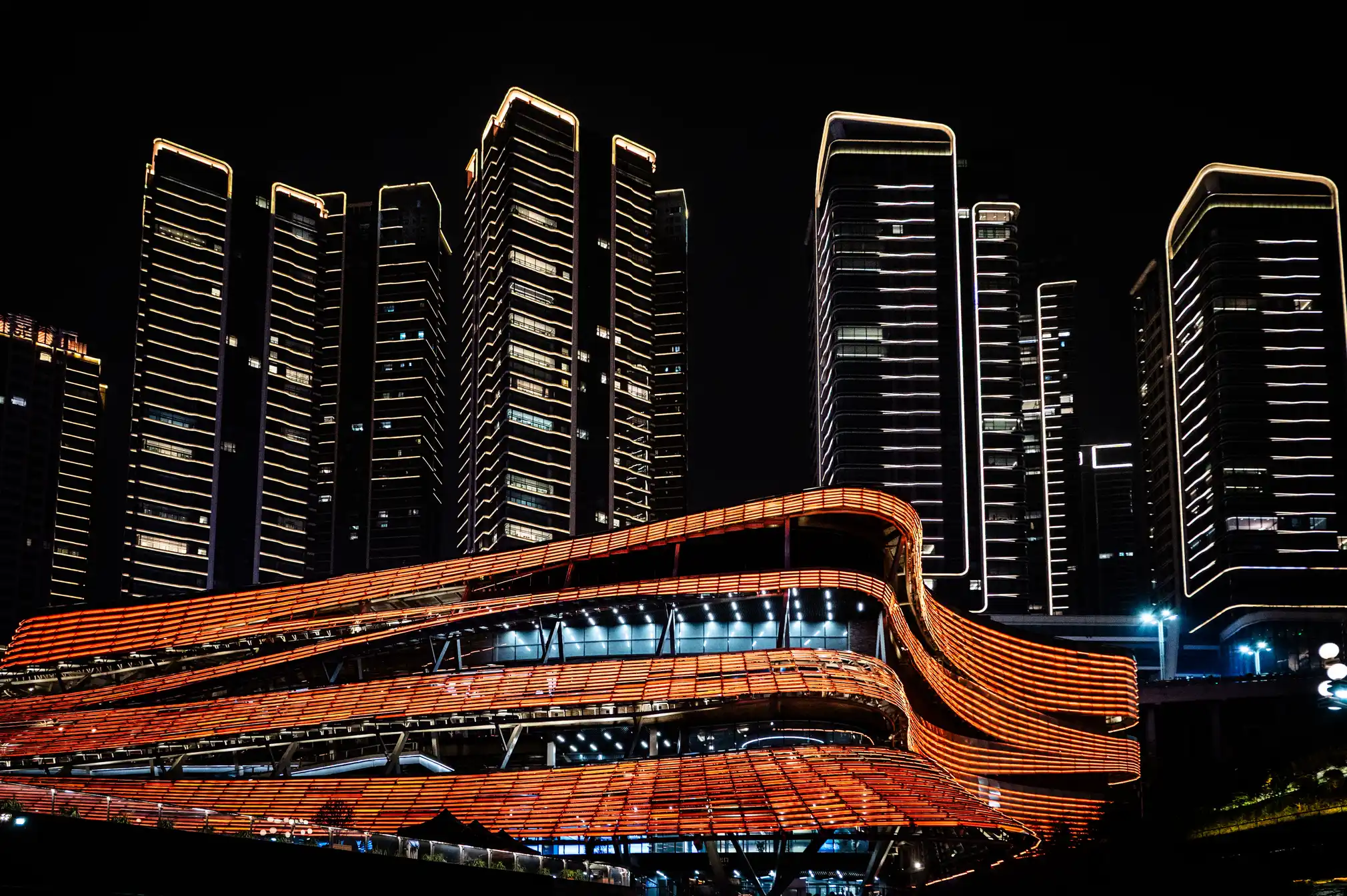
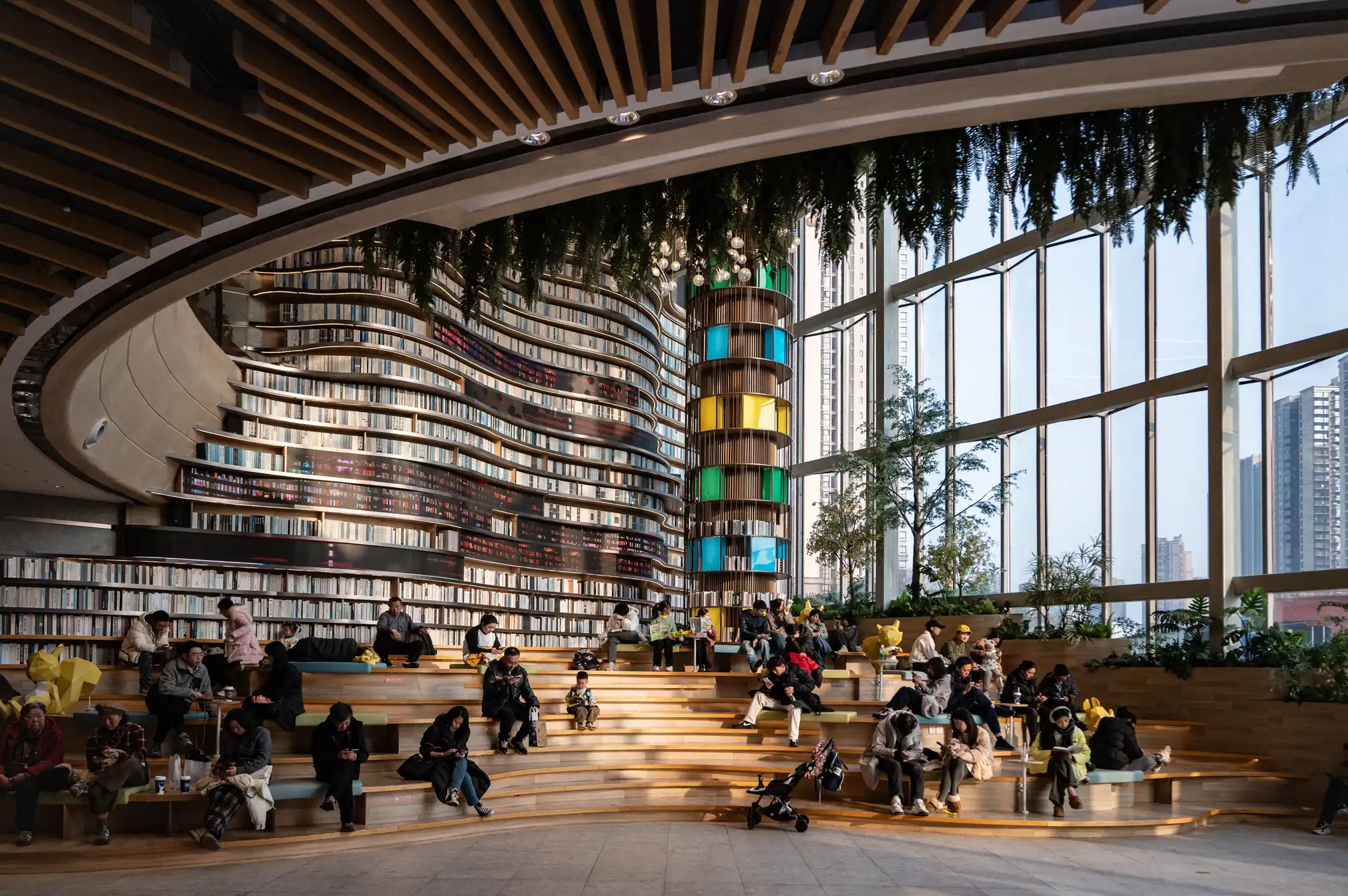
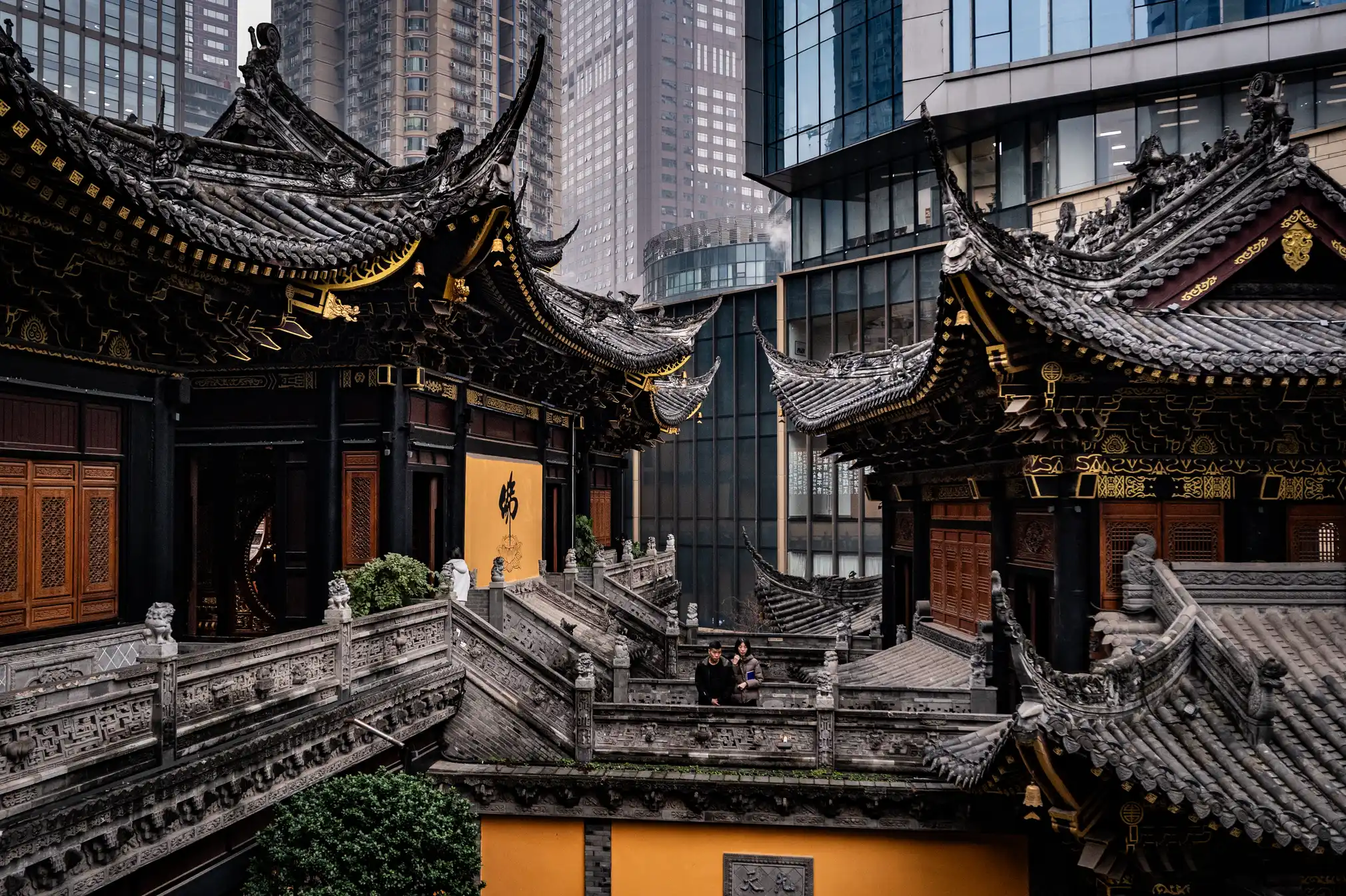
The largest city in the world is as big as Austria, but few people have ever heard of it. The megacity of 34 million people in central of China is the emblem of the fastest urban revolution on the planet.
I was working an album cover last night and got these really cool images in midjourney so made a video out of it. Animated using Pika. Song made using Suno Full version on my bandcamp. It’s called Static.
In HD we often refer to the range of available colors as a color gamut. Such a color gamut is typically plotted on a two-dimensional diagram, called a CIE chart, as shown in at the top of this blog. Each color is characterized by its x/y coordinates.
Good enough for government work, perhaps. But for HDR, with its higher luminance levels and wider color, the gamut becomes three-dimensional.
For HDR the color gamut therefore becomes a characteristic we now call the color volume. It isn’t easy to show color volume on a two-dimensional medium like the printed page or a computer screen, but one method is shown below. As the luminance becomes higher, the picture eventually turns to white. As it becomes darker, it fades to black. The traditional color gamut shown on the CIE chart is simply a slice through this color volume at a selected luminance level, such as 50%.
Three different color volumes—we still refer to them as color gamuts though their third dimension is important—are currently the most significant. The first is BT.709 (sometimes referred to as Rec.709), the color gamut used for pre-UHD/HDR formats, including standard HD.
The largest is known as BT.2020; it encompasses (roughly) the range of colors visible to the human eye (though ET might find it insufficient!).
Between these two is the color gamut used in digital cinema, known as DCI-P3.
Artificial light sources, not unlike the diverse phases of natural light, vary considerably in their properties. As a result, some lamps render an object’s color better than others do.
The most important criterion for assessing the color-rendering ability of any lamp is its spectral power distribution curve.
Natural daylight varies too much in strength and spectral composition to be taken seriously as a lighting standard for grading and dealing colored stones. For anything to be a standard, it must be constant in its properties, which natural light is not.
For dealers in particular to make the transition from natural light to an artificial light source, that source must offer:
1- A degree of illuminance at least as strong as the common phases of natural daylight.
2- Spectral properties identical or comparable to a phase of natural daylight.
A source combining these two things makes gems appear much the same as when viewed under a given phase of natural light. From the viewpoint of many dealers, this corresponds to a naturalappearance.
The 6000° Kelvin xenon short-arc lamp appears closest to meeting the criteria for a standard light source. Besides the strong illuminance this lamp affords, its spectrum is very similar to CIE standard illuminants of similar color temperature.
“Not every light performs the same way. Lights and lighting are tricky to handle. You have to plan for every circumstance. But the good news is, lighting can be adjusted. Let’s look at different factors that affect lighting in every scene you shoot. “
Use CRI, Luminous Efficacy and color temperature controls to match your needs.
Color Temperature Color temperature describes the “color” of white light by a light source radiated by a perfect black body at a given temperature measured in degrees Kelvin
CRI “The Color Rendering Index is a measurement of how faithfully a light source reveals the colors of whatever it illuminates, it describes the ability of a light source to reveal the color of an object, as compared to the color a natural light source would provide. The highest possible CRI is 100. A CRI of 100 generally refers to a perfect black body, like a tungsten light source or the sun. “
Black-body radiation is the type of electromagnetic radiation within or surrounding a body in thermodynamic equilibrium with its environment, or emitted by a black body (an opaque and non-reflective body) held at constant, uniform temperature. The radiation has a specific spectrum and intensity that depends only on the temperature of the body.
A black-body at room temperature appears black, as most of the energy it radiates is infra-red and cannot be perceived by the human eye. At higher temperatures, black bodies glow with increasing intensity and colors that range from dull red to blindingly brilliant blue-white as the temperature increases.
ACES 2.0 is the second major release of the components that make up the ACES system. The most significant change is a new suite of rendering transforms whose design was informed by collected feedback and requests from users of ACES 1. The changes aim to improve the appearance of perceived artifacts and to complete previously unfinished components of the system, resulting in a more complete, robust, and consistent product.
Highlights of the key changes in ACES 2.0 are as follows:
New output transforms, including:
A less aggressive tone scale
More intuitive controls to create custom outputs to non-standard displays
Robust gamut mapping to improve perceptual uniformity
Improved performance of the inverse transforms
Enhanced AMF specification
An updated specification for ACES Transform IDs
OpenEXR compression recommendations
Enhanced tools for generating Input Transforms and recommended procedures for characterizing prosumer cameras
Look Transform Library
Expanded documentation
Rendering Transform
The most substantial change in ACES 2.0 is a complete redesign of the rendering transform.
ACES 2.0 was built as a unified system, rather than through piecemeal additions. Different deliverable outputs “match” better and making outputs to display setups other than the provided presets is intended to be user-driven. The rendering transforms are less likely to produce undesirable artifacts “out of the box”, which means less time can be spent fixing problematic images and more time making pictures look the way you want.
Key design goals
Improve consistency of tone scale and provide an easy to use parameter to allow for outputs between preset dynamic ranges
Minimize hue skews across exposure range in a region of same hue
Unify for structural consistency across transform type
Easy to use parameters to create outputs other than the presets
Robust gamut mapping to improve harsh clipping artifacts
Fill extents of output code value cube (where appropriate and expected)
Invertible – not necessarily reversible, but Output > ACES > Output round-trip should be possible
Accomplish all of the above while maintaining an acceptable “out-of-the box” rendering
Chroma Key Green, the color of green screens is also known as Chroma Green and is valued at approximately 354C in the Pantone color matching system (PMS).
Chroma Green can be broken down in many different ways. Here is green screen green as other values useful for both physical and digital production:
Green Screen as RGB Color Value: 0, 177, 64
Green Screen as CMYK Color Value: 81, 0, 92, 0
Green Screen as Hex Color Value: #00b140
Green Screen as Websafe Color Value: #009933
Chroma Key Green is reasonably close to an 18% gray reflectance.
Illuminate your green screen with an uniform source with less than 2/3 EV variation.
The level of brightness at any given f-stop should be equivalent to a 90% white card under the same lighting.
Black-body radiation is the type of electromagnetic radiation within or surrounding a body in thermodynamic equilibrium with its environment, or emitted by a black body (an opaque and non-reflective body) held at constant, uniform temperature. The radiation has a specific spectrum and intensity that depends only on the temperature of the body.
A black-body at room temperature appears black, as most of the energy it radiates is infra-red and cannot be perceived by the human eye. At higher temperatures, black bodies glow with increasing intensity and colors that range from dull red to blindingly brilliant blue-white as the temperature increases.
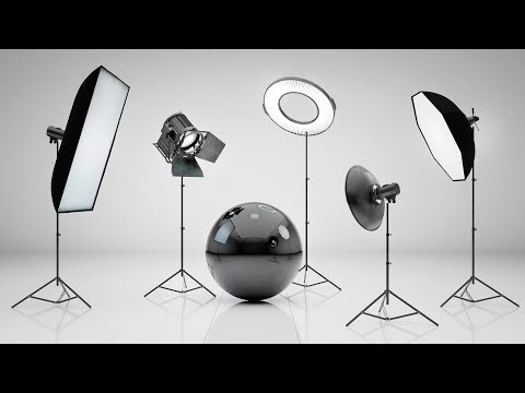
LightIt is a script for Maya and Arnold that will help you and improve your lighting workflow.
Thanks to preset studio lighting components (lights, backdrop…), high quality studio scenes and HDRI library manager.
RGBW (RGB + White) LED strip uses a 4-in-1 LED chip made up of red, green, blue, and white.
RGBWW (RGB + White + Warm White) LED strip uses either a 5-in-1 LED chip with red, green, blue, white, and warm white for color mixing. The only difference between RGBW and RGBWW is the intensity of the white color. The term RGBCCT consists of RGB and CCT. CCT (Correlated Color Temperature) means that the color temperature of the led strip light can be adjusted to change between warm white and white. Thus, RGBWW strip light is another name of RGBCCT strip.
RGBCW is the acronym for Red, Green, Blue, Cold, and Warm. These 5-in-1 chips are used in supper bright smart LED lighting products
An exposure stop is a unit measurement of Exposure as such it provides a universal linear scale to measure the increase and decrease in light, exposed to the image sensor, due to changes in shutter speed, iso and f-stop.
+-1 stop is a doubling or halving of the amount of light let in when taking a photo
1 EV (exposure value) is just another way to say one stop of exposure change.
Same applies to shutter speed, iso and aperture.
Doubling or halving your shutter speed produces an increase or decrease of 1 stop of exposure.
Doubling or halving your iso speed produces an increase or decrease of 1 stop of exposure.
DISCLAIMER – Links and images on this website may be protected by the respective owners’ copyright. All data submitted by users through this site shall be treated as freely available to share.