


COMPOSITION
DESIGN
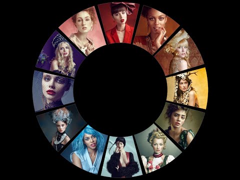
COLOR
-
What is a Gamut or Color Space and why do I need to know about CIE
Read more: What is a Gamut or Color Space and why do I need to know about CIE

http://www.xdcam-user.com/2014/05/what-is-a-gamut-or-color-space-and-why-do-i-need-to-know-about-it/
In video terms gamut is normally related to as the full range of colours and brightness that can be either captured or displayed.
Generally speaking all color gamuts recommendations are trying to define a reasonable level of color representation based on available technology and hardware. REC-601 represents the old TVs. REC-709 is currently the most distributed solution. P3 is mainly available in movie theaters and is now being adopted in some of the best new 4K HDR TVs. Rec2020 (a wider space than P3 that improves on visibke color representation) and ACES (the full coverage of visible color) are other common standards which see major hardware development these days.

To compare and visualize different solution (across video and printing solutions), most developers use the CIE color model chart as a reference.
The CIE color model is a color space model created by the International Commission on Illumination known as the Commission Internationale de l’Elcairage (CIE) in 1931. It is also known as the CIE XYZ color space or the CIE 1931 XYZ color space.
This chart represents the first defined quantitative link between distributions of wavelengths in the electromagnetic visible spectrum, and physiologically perceived colors in human color vision. Or basically, the range of color a typical human eye can perceive through visible light.
Note that while the human perception is quite wide, and generally speaking biased towards greens (we are apes after all), the amount of colors available through nature, generated through light reflection, tend to be a much smaller section. This is defined by the Pointer’s Chart.


In short. Color gamut is a representation of color coverage, used to describe data stored in images against available hardware and viewer technologies.
Camera color encoding from
https://www.slideshare.net/hpduiker/acescg-a-common-color-encoding-for-visual-effects-applications
CIE 1976
http://bernardsmith.eu/computatrum/scan_and_restore_archive_and_print/scanning/
https://store.yujiintl.com/blogs/high-cri-led/understanding-cie1931-and-cie-1976
The CIE 1931 standard has been replaced by a CIE 1976 standard. Below we can see the significance of this.
People have observed that the biggest issue with CIE 1931 is the lack of uniformity with chromaticity, the three dimension color space in rectangular coordinates is not visually uniformed.
The CIE 1976 (also called CIELUV) was created by the CIE in 1976. It was put forward in an attempt to provide a more uniform color spacing than CIE 1931 for colors at approximately the same luminance
The CIE 1976 standard colour space is more linear and variations in perceived colour between different people has also been reduced. The disproportionately large green-turquoise area in CIE 1931, which cannot be generated with existing computer screens, has been reduced.
If we move from CIE 1931 to the CIE 1976 standard colour space we can see that the improvements made in the gamut for the “new” iPad screen (as compared to the “old” iPad 2) are more evident in the CIE 1976 colour space than in the CIE 1931 colour space, particularly in the blues from aqua to deep blue.

https://dot-color.com/2012/08/14/color-space-confusion/
Despite its age, CIE 1931, named for the year of its adoption, remains a well-worn and familiar shorthand throughout the display industry. CIE 1931 is the primary language of customers. When a customer says that their current display “can do 72% of NTSC,” they implicitly mean 72% of NTSC 1953 color gamut as mapped against CIE 1931.
-
Björn Ottosson – OKHSV and OKHSL – Two new color spaces for color picking
Read more: Björn Ottosson – OKHSV and OKHSL – Two new color spaces for color pickinghttps://bottosson.github.io/misc/colorpicker
https://bottosson.github.io/posts/colorpicker/
https://www.smashingmagazine.com/2024/10/interview-bjorn-ottosson-creator-oklab-color-space/
One problem with sRGB is that in a gradient between blue and white, it becomes a bit purple in the middle of the transition. That’s because sRGB really isn’t created to mimic how the eye sees colors; rather, it is based on how CRT monitors work. That means it works with certain frequencies of red, green, and blue, and also the non-linear coding called gamma. It’s a miracle it works as well as it does, but it’s not connected to color perception. When using those tools, you sometimes get surprising results, like purple in the gradient.

There were also attempts to create simple models matching human perception based on XYZ, but as it turned out, it’s not possible to model all color vision that way. Perception of color is incredibly complex and depends, among other things, on whether it is dark or light in the room and the background color it is against. When you look at a photograph, it also depends on what you think the color of the light source is. The dress is a typical example of color vision being very context-dependent. It is almost impossible to model this perfectly.
I based Oklab on two other color spaces, CIECAM16 and IPT. I used the lightness and saturation prediction from CIECAM16, which is a color appearance model, as a target. I actually wanted to use the datasets used to create CIECAM16, but I couldn’t find them.
IPT was designed to have better hue uniformity. In experiments, they asked people to match light and dark colors, saturated and unsaturated colors, which resulted in a dataset for which colors, subjectively, have the same hue. IPT has a few other issues but is the basis for hue in Oklab.
In the Munsell color system, colors are described with three parameters, designed to match the perceived appearance of colors: Hue, Chroma and Value. The parameters are designed to be independent and each have a uniform scale. This results in a color solid with an irregular shape. The parameters are designed to be independent and each have a uniform scale. This results in a color solid with an irregular shape. Modern color spaces and models, such as CIELAB, Cam16 and Björn Ottosson own Oklab, are very similar in their construction.

By far the most used color spaces today for color picking are HSL and HSV, two representations introduced in the classic 1978 paper “Color Spaces for Computer Graphics”. HSL and HSV designed to roughly correlate with perceptual color properties while being very simple and cheap to compute.
Today HSL and HSV are most commonly used together with the sRGB color space.

One of the main advantages of HSL and HSV over the different Lab color spaces is that they map the sRGB gamut to a cylinder. This makes them easy to use since all parameters can be changed independently, without the risk of creating colors outside of the target gamut.

The main drawback on the other hand is that their properties don’t match human perception particularly well.
Reconciling these conflicting goals perfectly isn’t possible, but given that HSV and HSL don’t use anything derived from experiments relating to human perception, creating something that makes a better tradeoff does not seem unreasonable.
With this new lightness estimate, we are ready to look into the construction of Okhsv and Okhsl.


-
Photography Basics : Spectral Sensitivity Estimation Without a Camera
Read more: Photography Basics : Spectral Sensitivity Estimation Without a Camerahttps://color-lab-eilat.github.io/Spectral-sensitivity-estimation-web/
A number of problems in computer vision and related fields would be mitigated if camera spectral sensitivities were known. As consumer cameras are not designed for high-precision visual tasks, manufacturers do not disclose spectral sensitivities. Their estimation requires a costly optical setup, which triggered researchers to come up with numerous indirect methods that aim to lower cost and complexity by using color targets. However, the use of color targets gives rise to new complications that make the estimation more difficult, and consequently, there currently exists no simple, low-cost, robust go-to method for spectral sensitivity estimation that non-specialized research labs can adopt. Furthermore, even if not limited by hardware or cost, researchers frequently work with imagery from multiple cameras that they do not have in their possession.
To provide a practical solution to this problem, we propose a framework for spectral sensitivity estimation that not only does not require any hardware (including a color target), but also does not require physical access to the camera itself. Similar to other work, we formulate an optimization problem that minimizes a two-term objective function: a camera-specific term from a system of equations, and a universal term that bounds the solution space.
Different than other work, we utilize publicly available high-quality calibration data to construct both terms. We use the colorimetric mapping matrices provided by the Adobe DNG Converter to formulate the camera-specific system of equations, and constrain the solutions using an autoencoder trained on a database of ground-truth curves. On average, we achieve reconstruction errors as low as those that can arise due to manufacturing imperfections between two copies of the same camera. We provide predicted sensitivities for more than 1,000 cameras that the Adobe DNG Converter currently supports, and discuss which tasks can become trivial when camera responses are available.


-
Is it possible to get a dark yellow
Read more: Is it possible to get a dark yellowhttps://www.patreon.com/posts/102660674
https://www.linkedin.com/posts/stephenwestland_here-is-a-post-about-the-dark-yellow-problem-activity-7187131643764092929-7uCL


-
Space bodies’ components and light spectroscopy
Read more: Space bodies’ components and light spectroscopywww.plutorules.com/page-111-space-rocks.html
This help’s us understand the composition of components in/on solar system bodies.
Dips in the observed light spectrum, also known as, lines of absorption occur as gasses absorb energy from light at specific points along the light spectrum.
These dips or darkened zones (lines of absorption) leave a finger print which identify elements and compounds.
In this image the dark absorption bands appear as lines of emission which occur as the result of emitted not reflected (absorbed) light.
Lines of absorption
 Lines of emission


-
Brett Jones / Phil Reyneri (Lightform) / Philipp7pc: The study of Projection Mapping through Projectors
Read more: Brett Jones / Phil Reyneri (Lightform) / Philipp7pc: The study of Projection Mapping through Projectors


Video Projection Tool Software
https://hcgilje.wordpress.com/vpt/
https://www.projectorpoint.co.uk/news/how-bright-should-my-projector-be/
http://www.adwindowscreens.com/the_calculator/
heavym
https://heavym.net/en/
MadMapper
https://madmapper.com/
-
HDR and Color
Read more: HDR and Colorhttps://www.soundandvision.com/content/nits-and-bits-hdr-and-color
In HD we often refer to the range of available colors as a color gamut. Such a color gamut is typically plotted on a two-dimensional diagram, called a CIE chart, as shown in at the top of this blog. Each color is characterized by its x/y coordinates.

Good enough for government work, perhaps. But for HDR, with its higher luminance levels and wider color, the gamut becomes three-dimensional.

For HDR the color gamut therefore becomes a characteristic we now call the color volume. It isn’t easy to show color volume on a two-dimensional medium like the printed page or a computer screen, but one method is shown below. As the luminance becomes higher, the picture eventually turns to white. As it becomes darker, it fades to black. The traditional color gamut shown on the CIE chart is simply a slice through this color volume at a selected luminance level, such as 50%.
Three different color volumes—we still refer to them as color gamuts though their third dimension is important—are currently the most significant. The first is BT.709 (sometimes referred to as Rec.709), the color gamut used for pre-UHD/HDR formats, including standard HD.
The largest is known as BT.2020; it encompasses (roughly) the range of colors visible to the human eye (though ET might find it insufficient!).
Between these two is the color gamut used in digital cinema, known as DCI-P3.

sRGB

D65

-
Weta Digital – Manuka Raytracer and Gazebo GPU renderers – pipeline
Read more: Weta Digital – Manuka Raytracer and Gazebo GPU renderers – pipelinehttps://jo.dreggn.org/home/2018_manuka.pdf
http://www.fxguide.com/featured/manuka-weta-digitals-new-renderer/

The Manuka rendering architecture has been designed in the spirit of the classic reyes rendering architecture. In its core, reyes is based on stochastic rasterisation of micropolygons, facilitating depth of field, motion blur, high geometric complexity,and programmable shading.
This is commonly achieved with Monte Carlo path tracing, using a paradigm often called shade-on-hit, in which the renderer alternates tracing rays with running shaders on the various ray hits. The shaders take the role of generating the inputs of the local material structure which is then used bypath sampling logic to evaluate contributions and to inform what further rays to cast through the scene.
Over the years, however, the expectations have risen substantially when it comes to image quality. Computing pictures which are indistinguishable from real footage requires accurate simulation of light transport, which is most often performed using some variant of Monte Carlo path tracing. Unfortunately this paradigm requires random memory accesses to the whole scene and does not lend itself well to a rasterisation approach at all.
Manuka is both a uni-directional and bidirectional path tracer and encompasses multiple importance sampling (MIS). Interestingly, and importantly for production character skin work, it is the first major production renderer to incorporate spectral MIS in the form of a new ‘Hero Spectral Sampling’ technique, which was recently published at Eurographics Symposium on Rendering 2014.
Manuka propose a shade-before-hit paradigm in-stead and minimise I/O strain (and some memory costs) on the system, leveraging locality of reference by running pattern generation shaders before we execute light transport simulation by path sampling, “compressing” any bvh structure as needed, and as such also limiting duplication of source data.
The difference with reyes is that instead of baking colors into the geometry like in Reyes, manuka bakes surface closures. This means that light transport is still calculated with path tracing, but all texture lookups etc. are done up-front and baked into the geometry.The main drawback with this method is that geometry has to be tessellated to its highest, stable topology before shading can be evaluated properly. As such, the high cost to first pixel. Even a basic 4 vertices square becomes a much more complex model with this approach.

Manuka use the RenderMan Shading Language (rsl) for programmable shading [Pixar Animation Studios 2015], but we do not invoke rsl shaders when intersecting a ray with a surface (often called shade-on-hit). Instead, we pre-tessellate and pre-shade all the input geometry in the front end of the renderer.
This way, we can efficiently order shading computations to sup-port near-optimal texture locality, vectorisation, and parallelism. This system avoids repeated evaluation of shaders at the same surface point, and presents a minimal amount of memory to be accessed during light transport time. An added benefit is that the acceleration structure for ray tracing (abounding volume hierarchy, bvh) is built once on the final tessellated geometry, which allows us to ray trace more efficiently than multi-level bvhs and avoids costly caching of on-demand tessellated micropolygons and the associated scheduling issues.For the shading reasons above, in terms of AOVs, the studio approach is to succeed at combining complex shading with ray paths in the render rather than pass a multi-pass render to compositing.
For the Spectral Rendering component. The light transport stage is fully spectral, using a continuously sampled wavelength which is traced with each path and used to apply the spectral camera sensitivity of the sensor. This allows for faithfully support any degree of observer metamerism as the camera footage they are intended to match as well as complex materials which require wavelength dependent phenomena such as diffraction, dispersion, interference, iridescence, or chromatic extinction and Rayleigh scattering in participating media.
As opposed to the original reyes paper, we use bilinear interpolation of these bsdf inputs later when evaluating bsdfs per pathv ertex during light transport4. This improves temporal stability of geometry which moves very slowly with respect to the pixel raster
In terms of the pipeline, everything rendered at Weta was already completely interwoven with their deep data pipeline. Manuka very much was written with deep data in mind. Here, Manuka not so much extends the deep capabilities, rather it fully matches the already extremely complex and powerful setup Weta Digital already enjoy with RenderMan. For example, an ape in a scene can be selected, its ID is available and a NUKE artist can then paint in 3D say a hand and part of the way up the neutral posed ape.
We called our system Manuka, as a respectful nod to reyes: we had heard a story froma former ILM employee about how reyes got its name from how fond the early Pixar people were of their lunches at Point Reyes, and decided to name our system after our surrounding natural environment, too. Manuka is a kind of tea tree very common in New Zealand which has very many very small leaves, in analogy to micropolygons ina tree structure for ray tracing. It also happens to be the case that Weta Digital’s main site is on Manuka Street.


LIGHTING
-
GretagMacbeth Color Checker Numeric Values and Middle Gray
Read more: GretagMacbeth Color Checker Numeric Values and Middle GrayThe human eye perceives half scene brightness not as the linear 50% of the present energy (linear nature values) but as 18% of the overall brightness. We are biased to perceive more information in the dark and contrast areas. A Macbeth chart helps with calibrating back into a photographic capture into this “human perspective” of the world.
https://en.wikipedia.org/wiki/Middle_gray
In photography, painting, and other visual arts, middle gray or middle grey is a tone that is perceptually about halfway between black and white on a lightness scale in photography and printing, it is typically defined as 18% reflectance in visible light

Light meters, cameras, and pictures are often calibrated using an 18% gray card[4][5][6] or a color reference card such as a ColorChecker. On the assumption that 18% is similar to the average reflectance of a scene, a grey card can be used to estimate the required exposure of the film.
https://en.wikipedia.org/wiki/ColorChecker
(more…) -
Narcis Calin’s Galaxy Engine – A free, open source simulation software
Read more: Narcis Calin’s Galaxy Engine – A free, open source simulation softwareThis 2025 I decided to start learning how to code, so I installed Visual Studio and I started looking into C++. After days of watching tutorials and guides about the basics of C++ and programming, I decided to make something physics-related. I started with a dot that fell to the ground and then I wanted to simulate gravitational attraction, so I made 2 circles attracting each other. I thought it was really cool to see something I made with code actually work, so I kept building on top of that small, basic program. And here we are after roughly 8 months of learning programming. This is Galaxy Engine, and it is a simulation software I have been making ever since I started my learning journey. It currently can simulate gravity, dark matter, galaxies, the Big Bang, temperature, fluid dynamics, breakable solids, planetary interactions, etc. The program can run many tens of thousands of particles in real time on the CPU thanks to the Barnes-Hut algorithm, mixed with Morton curves. It also includes its own PBR 2D path tracer with BVH optimizations. The path tracer can simulate a bunch of stuff like diffuse lighting, specular reflections, refraction, internal reflection, fresnel, emission, dispersion, roughness, IOR, nested IOR and more! I tried to make the path tracer closer to traditional 3D render engines like V-Ray. I honestly never imagined I would go this far with programming, and it has been an amazing learning experience so far. I think that mixing this knowledge with my 3D knowledge can unlock countless new possibilities. In case you are curious about Galaxy Engine, I made it completely free and Open-Source so that anyone can build and compile it locally! You can find the source code in GitHub
https://github.com/NarcisCalin/Galaxy-Engine
-
Composition – 5 tips for creating perfect cinematic lighting and making your work look stunning
Read more: Composition – 5 tips for creating perfect cinematic lighting and making your work look stunning
http://www.diyphotography.net/5-tips-creating-perfect-cinematic-lighting-making-work-look-stunning/
1. Learn the rules of lighting
2. Learn when to break the rules
3. Make your key light larger
4. Reverse keying
5. Always be backlighting
-
What’s the Difference Between Ray Casting, Ray Tracing, Path Tracing and Rasterization? Physical light tracing…
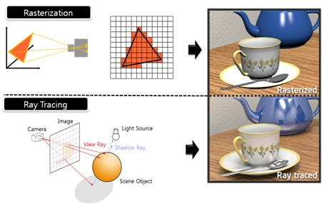
Read more: What’s the Difference Between Ray Casting, Ray Tracing, Path Tracing and Rasterization? Physical light tracing…RASTERIZATION
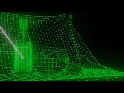
Rasterisation (or rasterization) is the task of taking the information described in a vector graphics format OR the vertices of triangles making 3D shapes and converting them into a raster image (a series of pixels, dots or lines, which, when displayed together, create the image which was represented via shapes), or in other words “rasterizing” vectors or 3D models onto a 2D plane for display on a computer screen.For each triangle of a 3D shape, you project the corners of the triangle on the virtual screen with some math (projective geometry). Then you have the position of the 3 corners of the triangle on the pixel screen. Those 3 points have texture coordinates, so you know where in the texture are the 3 corners. The cost is proportional to the number of triangles, and is only a little bit affected by the screen resolution.
In computer graphics, a raster graphics or bitmap image is a dot matrix data structure that represents a generally rectangular grid of pixels (points of color), viewable via a monitor, paper, or other display medium.
With rasterization, objects on the screen are created from a mesh of virtual triangles, or polygons, that create 3D models of objects. A lot of information is associated with each vertex, including its position in space, as well as information about color, texture and its “normal,” which is used to determine the way the surface of an object is facing.
Computers then convert the triangles of the 3D models into pixels, or dots, on a 2D screen. Each pixel can be assigned an initial color value from the data stored in the triangle vertices.
Further pixel processing or “shading,” including changing pixel color based on how lights in the scene hit the pixel, and applying one or more textures to the pixel, combine to generate the final color applied to a pixel.
The main advantage of rasterization is its speed. However, rasterization is simply the process of computing the mapping from scene geometry to pixels and does not prescribe a particular way to compute the color of those pixels. So it cannot take shading, especially the physical light, into account and it cannot promise to get a photorealistic output. That’s a big limitation of rasterization.
There are also multiple problems:
If you have two triangles one is behind the other, you will draw twice all the pixels. you only keep the pixel from the triangle that is closer to you (Z-buffer), but you still do the work twice.
The borders of your triangles are jagged as it is hard to know if a pixel is in the triangle or out. You can do some smoothing on those, that is anti-aliasing.
You have to handle every triangles (including the ones behind you) and then see that they do not touch the screen at all. (we have techniques to mitigate this where we only look at triangles that are in the field of view)
Transparency is hard to handle (you can’t just do an average of the color of overlapping transparent triangles, you have to do it in the right order)
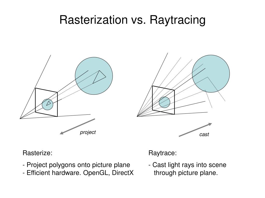
RAY CASTING
It is almost the exact reverse of rasterization: you start from the virtual screen instead of the vector or 3D shapes, and you project a ray, starting from each pixel of the screen, until it intersect with a triangle.The cost is directly correlated to the number of pixels in the screen and you need a really cheap way of finding the first triangle that intersect a ray. In the end, it is more expensive than rasterization but it will, by design, ignore the triangles that are out of the field of view.
You can use it to continue after the first triangle it hit, to take a little bit of the color of the next one, etc… This is useful to handle the border of the triangle cleanly (less jagged) and to handle transparency correctly.
RAYTRACING
Same idea as ray casting except once you hit a triangle you reflect on it and go into a different direction. The number of reflection you allow is the “depth” of your ray tracing. The color of the pixel can be calculated, based off the light source and all the polygons it had to reflect off of to get to that screen pixel.The easiest way to think of ray tracing is to look around you, right now. The objects you’re seeing are illuminated by beams of light. Now turn that around and follow the path of those beams backwards from your eye to the objects that light interacts with. That’s ray tracing.
Ray tracing is eye-oriented process that needs walking through each pixel looking for what object should be shown there, which is also can be described as a technique that follows a beam of light (in pixels) from a set point and simulates how it reacts when it encounters objects.
Compared with rasterization, ray tracing is hard to be implemented in real time, since even one ray can be traced and processed without much trouble, but after one ray bounces off an object, it can turn into 10 rays, and those 10 can turn into 100, 1000…The increase is exponential, and the the calculation for all these rays will be time consuming.
Historically, computer hardware hasn’t been fast enough to use these techniques in real time, such as in video games. Moviemakers can take as long as they like to render a single frame, so they do it offline in render farms. Video games have only a fraction of a second. As a result, most real-time graphics rely on the another technique called rasterization.
PATH TRACING
Path tracing can be used to solve more complex lighting situations.
Path tracing is a type of ray tracing. When using path tracing for rendering, the rays only produce a single ray per bounce. The rays do not follow a defined line per bounce (to a light, for example), but rather shoot off in a random direction. The path tracing algorithm then takes a random sampling of all of the rays to create the final image. This results in sampling a variety of different types of lighting.When a ray hits a surface it doesn’t trace a path to every light source, instead it bounces the ray off the surface and keeps bouncing it until it hits a light source or exhausts some bounce limit.
It then calculates the amount of light transferred all the way to the pixel, including any color information gathered from surfaces along the way.
It then averages out the values calculated from all the paths that were traced into the scene to get the final pixel color value.It requires a ton of computing power and if you don’t send out enough rays per pixel or don’t trace the paths far enough into the scene then you end up with a very spotty image as many pixels fail to find any light sources from their rays. So when you increase the the samples per pixel, you can see the image quality becomes better and better.
Ray tracing tends to be more efficient than path tracing. Basically, the render time of a ray tracer depends on the number of polygons in the scene. The more polygons you have, the longer it will take.
Meanwhile, the rendering time of a path tracer can be indifferent to the number of polygons, but it is related to light situation: If you add a light, transparency, translucence, or other shader effects, the path tracer will slow down considerably.
blogs.nvidia.com/blog/2018/03/19/whats-difference-between-ray-tracing-rasterization/
https://en.wikipedia.org/wiki/Rasterisation
https://www.quora.com/Whats-the-difference-between-ray-tracing-and-path-tracing
-
HDRI shooting and editing by Xuan Prada and Greg Zaal
Read more: HDRI shooting and editing by Xuan Prada and Greg Zaalwww.xuanprada.com/blog/2014/11/3/hdri-shooting
http://blog.gregzaal.com/2016/03/16/make-your-own-hdri/
http://blog.hdrihaven.com/how-to-create-high-quality-hdri/
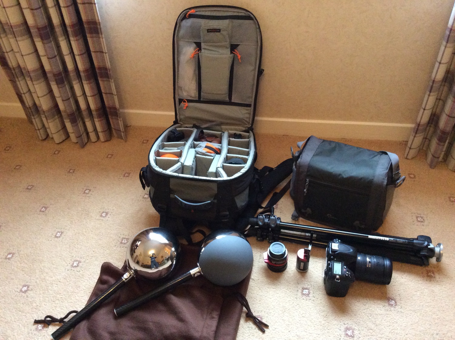
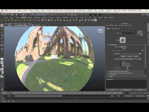
Shooting checklist
- Full coverage of the scene (fish-eye shots)
- Backplates for look-development (including ground or floor)
- Macbeth chart for white balance
- Grey ball for lighting calibration
- Chrome ball for lighting orientation
- Basic scene measurements
- Material samples
- Individual HDR artificial lighting sources if required
Methodology
(more…)


COLLECTIONS
| Featured AI
| Design And Composition
| Explore posts
POPULAR SEARCHES
unreal | pipeline | virtual production | free | learn | photoshop | 360 | macro | google | nvidia | resolution | open source | hdri | real-time | photography basics | nuke
FEATURED POSTS
Social Links
DISCLAIMER – Links and images on this website may be protected by the respective owners’ copyright. All data submitted by users through this site shall be treated as freely available to share.
