


COMPOSITION
-
Composition – These are the basic lighting techniques you need to know for photography and film
Read more: Composition – These are the basic lighting techniques you need to know for photography and film
http://www.diyphotography.net/basic-lighting-techniques-need-know-photography-film/
Amongst the basic techniques, there’s…
1- Side lighting – Literally how it sounds, lighting a subject from the side when they’re faced toward you
2- Rembrandt lighting – Here the light is at around 45 degrees over from the front of the subject, raised and pointing down at 45 degrees
3- Back lighting – Again, how it sounds, lighting a subject from behind. This can help to add drama with silouettes
4- Rim lighting – This produces a light glowing outline around your subject
5- Key light – The main light source, and it’s not necessarily always the brightest light source
6- Fill light – This is used to fill in the shadows and provide detail that would otherwise be blackness
7- Cross lighting – Using two lights placed opposite from each other to light two subjects


DESIGN


COLOR
-
Virtual Production volumes study
Read more: Virtual Production volumes studyColor Fidelity in LED Volumes
https://theasc.com/articles/color-fidelity-in-led-volumes
Virtual Production Glossary
https://vpglossary.com/What is Virtual Production – In depth analysis
https://www.leadingledtech.com/what-is-a-led-virtual-production-studio-in-depth-technical-analysis/
A comparison of LED panels for use in Virtual Production:
Findings and recommendations
https://eprints.bournemouth.ac.uk/36826/1/LED_Comparison_White_Paper%281%29.pdf -
About color: What is a LUT
Read more: About color: What is a LUThttp://www.lightillusion.com/luts.html
https://www.shutterstock.com/blog/how-use-luts-color-grading
A LUT (Lookup Table) is essentially the modifier between two images, the original image and the displayed image, based on a mathematical formula. Basically conversion matrices of different complexities. There are different types of LUTS – viewing, transform, calibration, 1D and 3D.


-
StudioBinder.com – CRI color rendering index
Read more: StudioBinder.com – CRI color rendering indexwww.studiobinder.com/blog/what-is-color-rendering-index
“The Color Rendering Index is a measurement of how faithfully a light source reveals the colors of whatever it illuminates, it describes the ability of a light source to reveal the color of an object, as compared to the color a natural light source would provide. The highest possible CRI is 100. A CRI of 100 generally refers to a perfect black body, like a tungsten light source or the sun. ”


www.pixelsham.com/2021/04/28/types-of-film-lights-and-their-efficiency
-
Practical Aspects of Spectral Data and LEDs in Digital Content Production and Virtual Production – SIGGRAPH 2022
Read more: Practical Aspects of Spectral Data and LEDs in Digital Content Production and Virtual Production – SIGGRAPH 2022
Comparison to the commercial side

https://www.ecolorled.com/blog/detail/what-is-rgb-rgbw-rgbic-strip-lights
RGBW (RGB + White) LED strip uses a 4-in-1 LED chip made up of red, green, blue, and white.
RGBWW (RGB + White + Warm White) LED strip uses either a 5-in-1 LED chip with red, green, blue, white, and warm white for color mixing. The only difference between RGBW and RGBWW is the intensity of the white color. The term RGBCCT consists of RGB and CCT. CCT (Correlated Color Temperature) means that the color temperature of the led strip light can be adjusted to change between warm white and white. Thus, RGBWW strip light is another name of RGBCCT strip.
RGBCW is the acronym for Red, Green, Blue, Cold, and Warm. These 5-in-1 chips are used in supper bright smart LED lighting products
-
Christopher Butler – Understanding the Eye-Mind Connection – Vision is a mental process
Read more: Christopher Butler – Understanding the Eye-Mind Connection – Vision is a mental processhttps://www.chrbutler.com/understanding-the-eye-mind-connection
The intricate relationship between the eyes and the brain, often termed the eye-mind connection, reveals that vision is predominantly a cognitive process. This understanding has profound implications for fields such as design, where capturing and maintaining attention is paramount. This essay delves into the nuances of visual perception, the brain’s role in interpreting visual data, and how this knowledge can be applied to effective design strategies.
This cognitive aspect of vision is evident in phenomena such as optical illusions, where the brain interprets visual information in a way that contradicts physical reality. These illusions underscore that what we “see” is not merely a direct recording of the external world but a constructed experience shaped by cognitive processes.
Understanding the cognitive nature of vision is crucial for effective design. Designers must consider how the brain processes visual information to create compelling and engaging visuals. This involves several key principles:
- Attention and Engagement
- Visual Hierarchy
- Cognitive Load Management
- Context and Meaning


![[gamma correction test]](http://www.madore.org/~david/misc/color/gammatest.png "sRGB gamma correction test")


LIGHTING
-
Gamma correction
Read more: Gamma correction

http://www.normankoren.com/makingfineprints1A.html#Gammabox
https://en.wikipedia.org/wiki/Gamma_correction
http://www.photoscientia.co.uk/Gamma.htm
https://www.w3.org/Graphics/Color/sRGB.html
http://www.eizoglobal.com/library/basics/lcd_display_gamma/index.html
https://forum.reallusion.com/PrintTopic308094.aspx
Basically, gamma is the relationship between the brightness of a pixel as it appears on the screen, and the numerical value of that pixel. Generally Gamma is just about defining relationships.
Three main types:
– Image Gamma encoded in images
– Display Gammas encoded in hardware and/or viewing time
– System or Viewing Gamma which is the net effect of all gammas when you look back at a final image. In theory this should flatten back to 1.0 gamma.
(more…) -
Terminators and Iron Men: HDRI, Image-based lighting and physical shading at ILM – Siggraph 2010
Read more: Terminators and Iron Men: HDRI, Image-based lighting and physical shading at ILM – Siggraph 2010 -
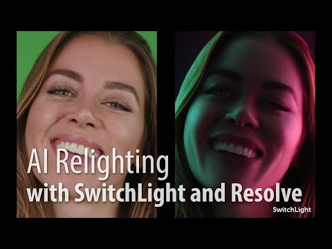
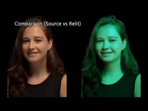
Beeble Switchlight’s Plugin for Foundry Nuke
Read more: Beeble Switchlight’s Plugin for Foundry Nukehttps://www.cutout.pro/learn/beeble-switchlight/
https://www.switchlight-api.beeble.ai/pricing
https://www.switchlight-api.beeble.ai
https://github.com/beeble-ai/SwitchLight-Studio
https://beeble.ai/terms-of-use
https://www.switchlight-api.beeble.ai/docs
-
DiffusionLight: HDRI Light Probes for Free by Painting a Chrome Ball
Read more: DiffusionLight: HDRI Light Probes for Free by Painting a Chrome Ballhttps://diffusionlight.github.io/
https://github.com/DiffusionLight/DiffusionLight
https://github.com/DiffusionLight/DiffusionLight?tab=MIT-1-ov-file#readme
https://colab.research.google.com/drive/15pC4qb9mEtRYsW3utXkk-jnaeVxUy-0S
“a simple yet effective technique to estimate lighting in a single input image. Current techniques rely heavily on HDR panorama datasets to train neural networks to regress an input with limited field-of-view to a full environment map. However, these approaches often struggle with real-world, uncontrolled settings due to the limited diversity and size of their datasets. To address this problem, we leverage diffusion models trained on billions of standard images to render a chrome ball into the input image. Despite its simplicity, this task remains challenging: the diffusion models often insert incorrect or inconsistent objects and cannot readily generate images in HDR format. Our research uncovers a surprising relationship between the appearance of chrome balls and the initial diffusion noise map, which we utilize to consistently generate high-quality chrome balls. We further fine-tune an LDR difusion model (Stable Diffusion XL) with LoRA, enabling it to perform exposure bracketing for HDR light estimation. Our method produces convincing light estimates across diverse settings and demonstrates superior generalization to in-the-wild scenarios.”

-
Black Body color aka the Planckian Locus curve for white point eye perception
Read more: Black Body color aka the Planckian Locus curve for white point eye perceptionhttp://en.wikipedia.org/wiki/Black-body_radiation

Black-body radiation is the type of electromagnetic radiation within or surrounding a body in thermodynamic equilibrium with its environment, or emitted by a black body (an opaque and non-reflective body) held at constant, uniform temperature. The radiation has a specific spectrum and intensity that depends only on the temperature of the body.
A black-body at room temperature appears black, as most of the energy it radiates is infra-red and cannot be perceived by the human eye. At higher temperatures, black bodies glow with increasing intensity and colors that range from dull red to blindingly brilliant blue-white as the temperature increases.
(more…) -
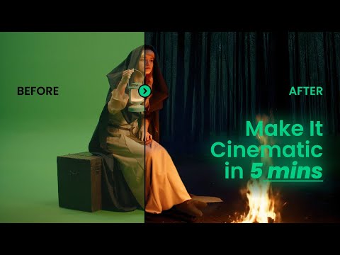
9 Best Hacks to Make a Cinematic Video with Any Camera
Read more: 9 Best Hacks to Make a Cinematic Video with Any Camerahttps://www.flexclip.com/learn/cinematic-video.html
- Frame Your Shots to Create Depth
- Create Shallow Depth of Field
- Avoid Shaky Footage and Use Flexible Camera Movements
- Properly Use Slow Motion
- Use Cinematic Lighting Techniques
- Apply Color Grading
- Use Cinematic Music and SFX
- Add Cinematic Fonts and Text Effects
- Create the Cinematic Bar at the Top and the Bottom

-
Types of Film Lights and their efficiency – CRI, Color Temperature and Luminous Efficacy
Read more: Types of Film Lights and their efficiency – CRI, Color Temperature and Luminous Efficacynofilmschool.com/types-of-film-lights
“Not every light performs the same way. Lights and lighting are tricky to handle. You have to plan for every circumstance. But the good news is, lighting can be adjusted. Let’s look at different factors that affect lighting in every scene you shoot. “
Use CRI, Luminous Efficacy and color temperature controls to match your needs.
Color Temperature
Color temperature describes the “color” of white light by a light source radiated by a perfect black body at a given temperature measured in degrees Kelvinhttps://www.pixelsham.com/2019/10/18/color-temperature/
CRI
“The Color Rendering Index is a measurement of how faithfully a light source reveals the colors of whatever it illuminates, it describes the ability of a light source to reveal the color of an object, as compared to the color a natural light source would provide. The highest possible CRI is 100. A CRI of 100 generally refers to a perfect black body, like a tungsten light source or the sun. “https://www.studiobinder.com/blog/what-is-color-rendering-index
(more…) -
Is a MacBeth Colour Rendition Chart the Safest Way to Calibrate a Camera?
Read more: Is a MacBeth Colour Rendition Chart the Safest Way to Calibrate a Camera?www.colour-science.org/posts/the-colorchecker-considered-mostly-harmless/
“Unless you have all the relevant spectral measurements, a colour rendition chart should not be used to perform colour-correction of camera imagery but only for white balancing and relative exposure adjustments.”
“Using a colour rendition chart for colour-correction might dramatically increase error if the scene light source spectrum is different from the illuminant used to compute the colour rendition chart’s reference values.”
“other factors make using a colour rendition chart unsuitable for camera calibration:
– Uncontrolled geometry of the colour rendition chart with the incident illumination and the camera.
– Unknown sample reflectances and ageing as the colour of the samples vary with time.
– Low samples count.
– Camera noise and flare.
– Etc…“Those issues are well understood in the VFX industry, and when receiving plates, we almost exclusively use colour rendition charts to white balance and perform relative exposure adjustments, i.e. plate neutralisation.”
-
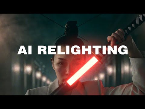
Magnific.ai Relight – change the entire lighting of a scene
Read more: Magnific.ai Relight – change the entire lighting of a scene
It’s a new Magnific spell that allows you to change the entire lighting of a scene and, optionally, the background with just:
1/ A prompt OR
2/ A reference image OR
3/ A light map (drawing your own lights)https://x.com/javilopen/status/1805274155065176489


COLLECTIONS
| Featured AI
| Design And Composition
| Explore posts
POPULAR SEARCHES
unreal | pipeline | virtual production | free | learn | photoshop | 360 | macro | google | nvidia | resolution | open source | hdri | real-time | photography basics | nuke
FEATURED POSTS
-
The Perils of Technical Debt – Understanding Its Impact on Security, Usability, and Stability
-
MiniTunes V1 – Free MP3 library app
-
Cinematographers Blueprint 300dpi poster
-
What’s the Difference Between Ray Casting, Ray Tracing, Path Tracing and Rasterization? Physical light tracing…
-
59 AI Filmmaking Tools For Your Workflow
-
GretagMacbeth Color Checker Numeric Values and Middle Gray
-
SourceTree vs Github Desktop – Which one to use
-
Convert 2D Images or Text to 3D Models
Social Links
DISCLAIMER – Links and images on this website may be protected by the respective owners’ copyright. All data submitted by users through this site shall be treated as freely available to share.
