slowmoVideo is an OpenSource program that creates slow-motion videos from your footage.
Slow motion cinematography is the result of playing back frames for a longer duration than they were exposed. For example, if you expose 240 frames of film in one second, then play them back at 24 fps, the resulting movie is 10 times longer (slower) than the original filmed event….
Film cameras are relatively simple mechanical devices that allow you to crank up the speed to whatever rate the shutter and pull-down mechanism allow. Some film cameras can operate at 2,500 fps or higher (although film shot in these cameras often needs some readjustment in postproduction). Video, on the other hand, is always captured, recorded, and played back at a fixed rate, with a current limit around 60fps. This makes extreme slow motion effects harder to achieve (and less elegant) on video, because slowing down the video results in each frame held still on the screen for a long time, whereas with high-frame-rate film there are plenty of frames to fill the longer durations of time. On video, the slow motion effect is more like a slide show than smooth, continuous motion.
One obvious solution is to shoot film at high speed, then transfer it to video (a case where film still has a clear advantage, sorry George). Another possibility is to cross dissolve or blur from one frame to the next. This adds a smooth transition from one still frame to the next. The blur reduces the sharpness of the image, and compared to slowing down images shot at a high frame rate, this is somewhat of a cheat. However, there isn’t much you can do about it until video can be recorded at much higher rates. Of course, many film cameras can’t shoot at high frame rates either, so the whole super-slow-motion endeavor is somewhat specialized no matter what medium you are using. (There are some high speed digital cameras available now that allow you to capture lots of digital frames directly to your computer, so technology is starting to catch up with film. However, this feature isn’t going to appear in consumer camcorders any time soon.)
To measure the contrast ratio you will need a light meter. The process starts with you measuring the main source of light, or the key light.
Get a reading from the brightest area on the face of your subject. Then, measure the area lit by the secondary light, or fill light. To make sense of what you have just measured you have to understand that the information you have just gathered is in F-stops, a measure of light. With each additional F-stop, for example going one stop from f/1.4 to f/2.0, you create a doubling of light. The reverse is also true; moving one stop from f/8.0 to f/5.6 results in a halving of the light.
Size. Mr. White (Harvey Keitel) on the right. Focus. He’s one of the two objects in focus. Lighting. Mr. White is large and in focus and Mr. Pink (Steve Buscemi) is highlighted by a shaft of light. Color. Both are black and white but the read on Mr. White’s shirt now really stands out.
The intricate relationship between the eyes and the brain, often termed the eye-mind connection, reveals that vision is predominantly a cognitive process. This understanding has profound implications for fields such as design, where capturing and maintaining attention is paramount. This essay delves into the nuances of visual perception, the brain’s role in interpreting visual data, and how this knowledge can be applied to effective design strategies.
This cognitive aspect of vision is evident in phenomena such as optical illusions, where the brain interprets visual information in a way that contradicts physical reality. These illusions underscore that what we “see” is not merely a direct recording of the external world but a constructed experience shaped by cognitive processes.
Understanding the cognitive nature of vision is crucial for effective design. Designers must consider how the brain processes visual information to create compelling and engaging visuals. This involves several key principles:
this is the epic story of a group of talented digital artists trying to overcame daily technical challenges to achieve incredibly photorealistic projects of monsters and aliens
By stimulating specific cells in the retina, the participants claim to have witnessed a blue-green colour that scientists have called “olo”, but some experts have said the existence of a new colour is “open to argument”.
The findings, published in the journal Science Advances on Friday, have been described by the study’s co-author, Prof Ren Ng from the University of California, as “remarkable”.
(A) System inputs. (i) Retina map of 103 cone cells preclassified by spectral type (7). (ii) Target visual percept (here, a video of a child, see movie S1 at 1:04). (iii) Infrared cellular-scale imaging of the retina with 60-frames-per-second rolling shutter. Fixational eye movement is visible over the three frames shown.
(B) System outputs. (iv) Real-time per-cone target activation levels to reproduce the target percept, computed by: extracting eye motion from the input video relative to the retina map; identifying the spectral type of every cone in the field of view; computing the per-cone activation the target percept would have produced. (v) Intensities of visible-wavelength 488-nm laser microdoses at each cone required to achieve its target activation level.
(C) Infrared imaging and visible-wavelength stimulation are physically accomplished in a raster scan across the retinal region using AOSLO. By modulating the visible-wavelength beam’s intensity, the laser microdoses shown in (v) are delivered. Drawing adapted with permission [Harmening and Sincich (54)].
(D) Examples of target percepts with corresponding cone activations and laser microdoses, ranging from colored squares to complex imagery. Teal-striped regions represent the color “olo” of stimulating only M cones.
Colour is an open-source Python package providing a comprehensive number of algorithms and datasets for colour science. It is freely available under the BSD-3-Clause terms.
The human eye perceives half scene brightness not as the linear 50% of the present energy (linear nature values) but as 18% of the overall brightness. We are biased to perceive more information in the dark and contrast areas. A Macbeth chart helps with calibrating back into a photographic capture into this “human perspective” of the world.
In photography, painting, and other visual arts, middle gray or middle grey is a tone that is perceptually about halfway between black and white on a lightness scale in photography and printing, it is typically defined as 18% reflectance in visible light
Light meters, cameras, and pictures are often calibrated using an 18% gray card[4][5][6] or a color reference card such as a ColorChecker. On the assumption that 18% is similar to the average reflectance of a scene, a grey card can be used to estimate the required exposure of the film.
The Manuka rendering architecture has been designed in the spirit of the classic reyes rendering architecture. In its core, reyes is based on stochastic rasterisation of micropolygons, facilitating depth of field, motion blur, high geometric complexity,and programmable shading.
This is commonly achieved with Monte Carlo path tracing, using a paradigm often called shade-on-hit, in which the renderer alternates tracing rays with running shaders on the various ray hits. The shaders take the role of generating the inputs of the local material structure which is then used bypath sampling logic to evaluate contributions and to inform what further rays to cast through the scene.
Over the years, however, the expectations have risen substantially when it comes to image quality. Computing pictures which are indistinguishable from real footage requires accurate simulation of light transport, which is most often performed using some variant of Monte Carlo path tracing. Unfortunately this paradigm requires random memory accesses to the whole scene and does not lend itself well to a rasterisation approach at all.
Manuka is both a uni-directional and bidirectional path tracer and encompasses multiple importance sampling (MIS). Interestingly, and importantly for production character skin work, it is the first major production renderer to incorporate spectral MIS in the form of a new ‘Hero Spectral Sampling’ technique, which was recently published at Eurographics Symposium on Rendering 2014.
Manuka propose a shade-before-hit paradigm in-stead and minimise I/O strain (and some memory costs) on the system, leveraging locality of reference by running pattern generation shaders before we execute light transport simulation by path sampling, “compressing” any bvh structure as needed, and as such also limiting duplication of source data.
The difference with reyes is that instead of baking colors into the geometry like in Reyes, manuka bakes surface closures. This means that light transport is still calculated with path tracing, but all texture lookups etc. are done up-front and baked into the geometry.
The main drawback with this method is that geometry has to be tessellated to its highest, stable topology before shading can be evaluated properly. As such, the high cost to first pixel. Even a basic 4 vertices square becomes a much more complex model with this approach.
Manuka use the RenderMan Shading Language (rsl) for programmable shading [Pixar Animation Studios 2015], but we do not invoke rsl shaders when intersecting a ray with a surface (often called shade-on-hit). Instead, we pre-tessellate and pre-shade all the input geometry in the front end of the renderer.
This way, we can efficiently order shading computations to sup-port near-optimal texture locality, vectorisation, and parallelism. This system avoids repeated evaluation of shaders at the same surface point, and presents a minimal amount of memory to be accessed during light transport time. An added benefit is that the acceleration structure for ray tracing (abounding volume hierarchy, bvh) is built once on the final tessellated geometry, which allows us to ray trace more efficiently than multi-level bvhs and avoids costly caching of on-demand tessellated micropolygons and the associated scheduling issues.
For the shading reasons above, in terms of AOVs, the studio approach is to succeed at combining complex shading with ray paths in the render rather than pass a multi-pass render to compositing.
For the Spectral Rendering component. The light transport stage is fully spectral, using a continuously sampled wavelength which is traced with each path and used to apply the spectral camera sensitivity of the sensor. This allows for faithfully support any degree of observer metamerism as the camera footage they are intended to match as well as complex materials which require wavelength dependent phenomena such as diffraction, dispersion, interference, iridescence, or chromatic extinction and Rayleigh scattering in participating media.
As opposed to the original reyes paper, we use bilinear interpolation of these bsdf inputs later when evaluating bsdfs per pathv ertex during light transport4. This improves temporal stability of geometry which moves very slowly with respect to the pixel raster
In terms of the pipeline, everything rendered at Weta was already completely interwoven with their deep data pipeline. Manuka very much was written with deep data in mind. Here, Manuka not so much extends the deep capabilities, rather it fully matches the already extremely complex and powerful setup Weta Digital already enjoy with RenderMan. For example, an ape in a scene can be selected, its ID is available and a NUKE artist can then paint in 3D say a hand and part of the way up the neutral posed ape.
We called our system Manuka, as a respectful nod to reyes: we had heard a story froma former ILM employee about how reyes got its name from how fond the early Pixar people were of their lunches at Point Reyes, and decided to name our system after our surrounding natural environment, too. Manuka is a kind of tea tree very common in New Zealand which has very many very small leaves, in analogy to micropolygons ina tree structure for ray tracing. It also happens to be the case that Weta Digital’s main site is on Manuka Street.
“The list should be helpful for every material artist who work on PBR materials as it contains over 200 color values measured with PCE-RGB2 1002 Color Spectrometer device and presented in linear and sRGB (2.2) gamma space.
All color values, HUE and Saturation in this list come from measurements taken with PCE-RGB2 1002 Color Spectrometer device and are presented in linear and sRGB (2.2) gamma space (more info at the end of this video) I calculated Relative Luminance and Luminance values based on captured color using my own equation which takes color based luminance perception into consideration. Bare in mind that there is no ‘one’ color per substance as nothing in nature is even 100% uniform and any value in +/-10% range from these should be considered as correct one. Therefore this list should be always considered as a color reference for material’s albedos, not ulitimate and absolute truth.“
Spectral sensitivity of eye is influenced by light intensity. And the light intensity determines the level of activity of cones cell and rod cell. This is the main characteristic of human vision. Sensitivity to individual colors, in other words, wavelengths of the light spectrum, is explained by the RGB (red-green-blue) theory. This theory assumed that there are three kinds of cones. It’s selectively sensitive to red (700-630 nm), green (560-500 nm), and blue (490-450 nm) light. And their mutual interaction allow to perceive all colors of the spectrum.
A measure of how large the object appears to an observer looking from that point. Thus. A measure for objects in the sky. Useful to retuen the size of the sun and moon… and in perspective, how much of their contribution to lighting. Solid angle can be represented in ‘angular diameter’ as well.
A solid angle is expressed in a dimensionless unit called a steradian (symbol: sr). By default in terms of the total celestial sphere and before atmospheric’s scattering, the Sun and the Moon subtend fractional areas of 0.000546% (Sun) and 0.000531% (Moon).
On earth the sun is likely closer to 0.00011 solid angle after athmospheric scattering. The sun as perceived from earth has a diameter of 0.53 degrees. This is about 0.000064 solid angle.
The mean angular diameter of the full moon is 2q = 0.52° (it varies with time around that average, by about 0.009°). This translates into a solid angle of 0.0000647 sr, which means that the whole night sky covers a solid angle roughly one hundred thousand times greater than the full moon.
The apparent size of an object as seen by an observer; expressed in units of degrees (of arc), arc minutes, or arc seconds. The moon, as viewed from the Earth, has an angular diameter of one-half a degree.
The angle covered by the diameter of the full moon is about 31 arcmin or 1/2°, so astronomers would say the Moon’s angular diameter is 31 arcmin, or the Moon subtends an angle of 31 arcmin.
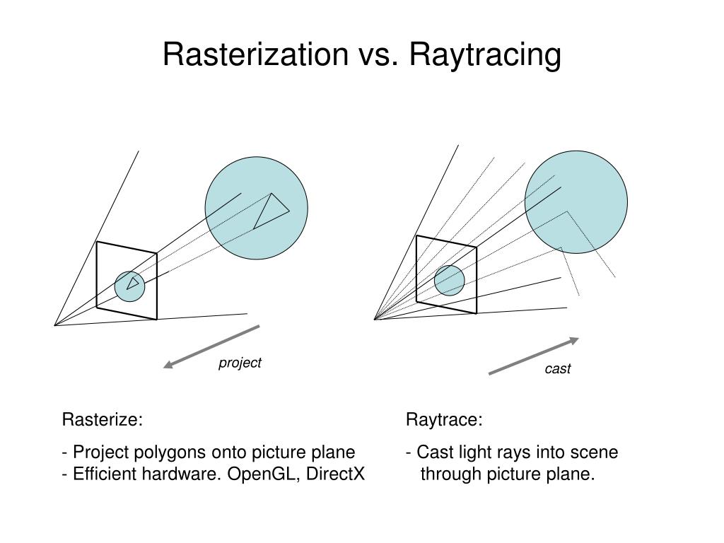
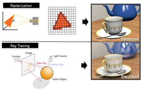
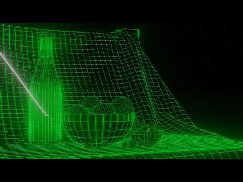
RASTERIZATION Rasterisation (or rasterization) is the task of taking the information described in a vector graphics format OR the vertices of triangles making 3D shapes and converting them into a raster image (a series of pixels, dots or lines, which, when displayed together, create the image which was represented via shapes), or in other words “rasterizing” vectors or 3D models onto a 2D plane for display on a computer screen.
For each triangle of a 3D shape, you project the corners of the triangle on the virtual screen with some math (projective geometry). Then you have the position of the 3 corners of the triangle on the pixel screen. Those 3 points have texture coordinates, so you know where in the texture are the 3 corners. The cost is proportional to the number of triangles, and is only a little bit affected by the screen resolution.
In computer graphics, a raster graphics orbitmap image is a dot matrix data structure that represents a generally rectangular grid of pixels (points of color), viewable via a monitor, paper, or other display medium.
With rasterization, objects on the screen are created from a mesh of virtual triangles, or polygons, that create 3D models of objects. A lot of information is associated with each vertex, including its position in space, as well as information about color, texture and its “normal,” which is used to determine the way the surface of an object is facing.
Computers then convert the triangles of the 3D models into pixels, or dots, on a 2D screen. Each pixel can be assigned an initial color value from the data stored in the triangle vertices.
Further pixel processing or “shading,” including changing pixel color based on how lights in the scene hit the pixel, and applying one or more textures to the pixel, combine to generate the final color applied to a pixel.
The main advantage of rasterization is its speed. However, rasterization is simply the process of computing the mapping from scene geometry to pixels and does not prescribe a particular way to compute the color of those pixels. So it cannot take shading, especially the physical light, into account and it cannot promise to get a photorealistic output. That’s a big limitation of rasterization.
There are also multiple problems:
If you have two triangles one is behind the other, you will draw twice all the pixels. you only keep the pixel from the triangle that is closer to you (Z-buffer), but you still do the work twice.
The borders of your triangles are jagged as it is hard to know if a pixel is in the triangle or out. You can do some smoothing on those, that is anti-aliasing.
You have to handle every triangles (including the ones behind you) and then see that they do not touch the screen at all. (we have techniques to mitigate this where we only look at triangles that are in the field of view)
Transparency is hard to handle (you can’t just do an average of the color of overlapping transparent triangles, you have to do it in the right order)
RAY CASTING It is almost the exact reverse of rasterization: you start from the virtual screen instead of the vector or 3D shapes, and you project a ray, starting from each pixel of the screen, until it intersect with a triangle.
The cost is directly correlated to the number of pixels in the screen and you need a really cheap way of finding the first triangle that intersect a ray. In the end, it is more expensive than rasterization but it will, by design, ignore the triangles that are out of the field of view.
You can use it to continue after the first triangle it hit, to take a little bit of the color of the next one, etc… This is useful to handle the border of the triangle cleanly (less jagged) and to handle transparency correctly.
RAYTRACING
Same idea as ray casting except once you hit a triangle you reflect on it and go into a different direction. The number of reflection you allow is the “depth” of your ray tracing. The color of the pixel can be calculated, based off the light source and all the polygons it had to reflect off of to get to that screen pixel.
The easiest way to think of ray tracing is to look around you, right now. The objects you’re seeing are illuminated by beams of light. Now turn that around and follow the path of those beams backwards from your eye to the objects that light interacts with. That’s ray tracing.
Ray tracing is eye-oriented process that needs walking through each pixel looking for what object should be shown there, which is also can be described as a technique that follows a beam of light (in pixels) from a set point and simulates how it reacts when it encounters objects.
Compared with rasterization, ray tracing is hard to be implemented in real time, since even one ray can be traced and processed without much trouble, but after one ray bounces off an object, it can turn into 10 rays, and those 10 can turn into 100, 1000…The increase is exponential, and the the calculation for all these rays will be time consuming.
Historically, computer hardware hasn’t been fast enough to use these techniques in real time, such as in video games. Moviemakers can take as long as they like to render a single frame, so they do it offline in render farms. Video games have only a fraction of a second. As a result, most real-time graphics rely on the another technique called rasterization.
PATH TRACING Path tracing can be used to solve more complex lighting situations. Path tracing is a type of ray tracing. When using path tracing for rendering, the rays only produce a single ray per bounce. The rays do not follow a defined line per bounce(to a light, for example), but rather shoot off in a random direction. The path tracing algorithm then takes a random sampling of all of the rays to create the final image. This results in sampling a variety of different types of lighting.
When a ray hits a surface it doesn’t trace a path to every light source, instead it bounces the ray off the surface and keeps bouncing it until it hits a light source or exhausts some bounce limit. It then calculates the amount of light transferred all the way to the pixel, including any color information gathered from surfaces along the way. It then averages out the values calculated from all the paths that were traced into the scene to get the final pixel color value.
It requires a ton of computing power and if you don’t send out enough rays per pixel or don’t trace the paths far enough into the scene then you end up with a very spotty image as many pixels fail to find any light sources from their rays. So when you increase the the samples per pixel, you can see the image quality becomes better and better.
Ray tracing tends to be more efficient than path tracing. Basically, the render time of a ray tracer depends on the number of polygons in the scene. The more polygons you have, the longer it will take. Meanwhile, the rendering time of a path tracer can be indifferent to the number of polygons, but it is related to light situation: If you add a light, transparency, translucence, or other shader effects, the path tracer will slow down considerably.
The trigger phrase is “equirectangular 360 degree panorama”. I would avoid saying “spherical projection” since that tends to result in non-equirectangular spherical images.
Image resolution should always be a 2:1 aspect ratio. 1024 x 512 or 1408 x 704 work quite well and were used in the training data. 2048 x 1024 also works.
I suggest using a weight of 0.5 – 1.5. If you are having issues with the image generating too flat instead of having the necessary spherical distortion, try increasing the weight above 1, though this could negatively impact small details of the image. For Flux guidance, I recommend a value of about 2.5 for realistic scenes.
DISCLAIMER – Links and images on this website may be protected by the respective owners’ copyright. All data submitted by users through this site shall be treated as freely available to share.


 Local copy:


