


COMPOSITION
-
7 Commandments of Film Editing and composition
Read more: 7 Commandments of Film Editing and composition
1. Watch every frame of raw footage twice. On the second time, take notes. If you don’t do this and try to start developing a scene premature, then it’s a big disservice to yourself and to the director, actors and production crew.
2. Nurture the relationships with the director. You are the secondary person in the relationship. Be calm and continually offer solutions. Get the main intention of the film as soon as possible from the director.
3. Organize your media so that you can find any shot instantly.
4. Factor in extra time for renders, exports, errors and crashes.
5. Attempt edits and ideas that shouldn’t work. It just might work. Until you do it and watch it, you won’t know. Don’t rule out ideas just because they don’t make sense in your mind.
6. Spend more time on your audio. It’s the glue of your edit. AUDIO SAVES EVERYTHING. Create fluid and seamless audio under your video.
7. Make cuts for the scene, but always in context for the whole film. Have a macro and a micro view at all times.
-
Composition – These are the basic lighting techniques you need to know for photography and film
Read more: Composition – These are the basic lighting techniques you need to know for photography and film
http://www.diyphotography.net/basic-lighting-techniques-need-know-photography-film/
Amongst the basic techniques, there’s…
1- Side lighting – Literally how it sounds, lighting a subject from the side when they’re faced toward you
2- Rembrandt lighting – Here the light is at around 45 degrees over from the front of the subject, raised and pointing down at 45 degrees
3- Back lighting – Again, how it sounds, lighting a subject from behind. This can help to add drama with silouettes
4- Rim lighting – This produces a light glowing outline around your subject
5- Key light – The main light source, and it’s not necessarily always the brightest light source
6- Fill light – This is used to fill in the shadows and provide detail that would otherwise be blackness
7- Cross lighting – Using two lights placed opposite from each other to light two subjects
-
Types of Film Lights and their efficiency – CRI, Color Temperature and Luminous Efficacy
Read more: Types of Film Lights and their efficiency – CRI, Color Temperature and Luminous Efficacynofilmschool.com/types-of-film-lights
“Not every light performs the same way. Lights and lighting are tricky to handle. You have to plan for every circumstance. But the good news is, lighting can be adjusted. Let’s look at different factors that affect lighting in every scene you shoot. “
Use CRI, Luminous Efficacy and color temperature controls to match your needs.
Color Temperature
Color temperature describes the “color” of white light by a light source radiated by a perfect black body at a given temperature measured in degrees Kelvinhttps://www.pixelsham.com/2019/10/18/color-temperature/
CRI
“The Color Rendering Index is a measurement of how faithfully a light source reveals the colors of whatever it illuminates, it describes the ability of a light source to reveal the color of an object, as compared to the color a natural light source would provide. The highest possible CRI is 100. A CRI of 100 generally refers to a perfect black body, like a tungsten light source or the sun. “https://www.studiobinder.com/blog/what-is-color-rendering-index
(more…)


DESIGN
-
VQGAN + CLIP AI made Music Video for the song Canvas by Resonate
Read more: VQGAN + CLIP AI made Music Video for the song Canvas by Resonate
” In this video, I utilized artificial intelligence to generate an animated music video for the song Canvas by Resonate. This tool allows anyone to generate beautiful images using only text as the input. My question was, what if I used song lyrics as input to the AI, can I make perfect music synchronized videos automatically with the push of a button? Let me know how you think the AI did in this visual interpretation of the song.
After getting caught up in the excitement around DALL·E2 (latest and greatest AI system, it’s INSANE), I searched for any way I could use similar image generation for music synchronization. Since DALL·E2 is not available to the public yet, my search led me to VQGAN + CLIP (Vector Quantized Generative Adversarial Network and Contrastive Language–Image Pre-training), before settling more specifically on Disco Diffusion V5.2 Turbo. If you don’t know what any of these words or acronyms mean, don’t worry, I was just as confused when I first started learning about this technology. I believe we’re reaching a turning point where entire industries are about to shift in reaction to this new process (which is essentially magic!).
DoodleChaos”
-
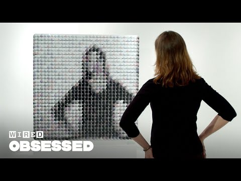
Pantheon of the War – The colossal war painting
Read more: Pantheon of the War – The colossal war paintingFour years in the making with the help of 150 artists, in commemoration of WW1.
edition.cnn.com/style/article/pantheon-de-la-guerre-wwi-painting/index.html
A panoramic canvas measuring 402 feet (122 meters) around and 45 feet (13.7 meters) high. It contained over 5,000 life-size portraits of war heroes, royalty and government officials from the Allies of World War I.
Partial section upload:


COLOR
-
Stefan Ringelschwandtner – LUT Inspector tool
Read more: Stefan Ringelschwandtner – LUT Inspector toolIt lets you load any .cube LUT right in your browser, see the RGB curves, and use a split view on the Granger Test Image to compare the original vs. LUT-applied version in real time — perfect for spotting hue shifts, saturation changes, and contrast tweaks.
https://mononodes.com/lut-inspector/


-
Yasuharu YOSHIZAWA – Comparison of sRGB vs ACREScg in Nuke
Read more: Yasuharu YOSHIZAWA – Comparison of sRGB vs ACREScg in NukeAnswering the question that is often asked, “Do I need to use ACEScg to display an sRGB monitor in the end?” (Demonstration shown at an in-house seminar)
Comparison of scanlineRender output with extreme color lights on color charts with sRGB/ACREScg in color – OCIO -working space in NukeDownload the Nuke script:
-
Pattern generators
Read more: Pattern generatorshttp://qrohlf.com/trianglify-generator/
https://halftonepro.com/app/polygons#
https://mattdesl.svbtle.com/generative-art-with-nodejs-and-canvas
https://www.patterncooler.com/
http://permadi.com/java/spaint/spaint.html
https://dribbble.com/shots/1847313-Kaleidoscope-Generator-PSD
http://eskimoblood.github.io/gerstnerizer/
http://www.stripegenerator.com/
http://btmills.github.io/geopattern/geopattern.html
http://fractalarchitect.net/FA4-Random-Generator.html
https://sciencevsmagic.net/fractal/#0605,0000,3,2,0,1,2
https://sites.google.com/site/mandelbulber/home
-
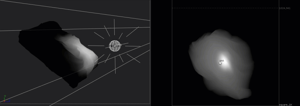
What light is best to illuminate gems for resale
Read more: What light is best to illuminate gems for resalewww.palagems.com/gem-lighting2
Artificial light sources, not unlike the diverse phases of natural light, vary considerably in their properties. As a result, some lamps render an object’s color better than others do.
The most important criterion for assessing the color-rendering ability of any lamp is its spectral power distribution curve.
Natural daylight varies too much in strength and spectral composition to be taken seriously as a lighting standard for grading and dealing colored stones. For anything to be a standard, it must be constant in its properties, which natural light is not.
For dealers in particular to make the transition from natural light to an artificial light source, that source must offer:
1- A degree of illuminance at least as strong as the common phases of natural daylight.
2- Spectral properties identical or comparable to a phase of natural daylight.A source combining these two things makes gems appear much the same as when viewed under a given phase of natural light. From the viewpoint of many dealers, this corresponds to a naturalappearance.
The 6000° Kelvin xenon short-arc lamp appears closest to meeting the criteria for a standard light source. Besides the strong illuminance this lamp affords, its spectrum is very similar to CIE standard illuminants of similar color temperature.


-
GretagMacbeth Color Checker Numeric Values and Middle Gray
Read more: GretagMacbeth Color Checker Numeric Values and Middle GrayThe human eye perceives half scene brightness not as the linear 50% of the present energy (linear nature values) but as 18% of the overall brightness. We are biased to perceive more information in the dark and contrast areas. A Macbeth chart helps with calibrating back into a photographic capture into this “human perspective” of the world.
https://en.wikipedia.org/wiki/Middle_gray
In photography, painting, and other visual arts, middle gray or middle grey is a tone that is perceptually about halfway between black and white on a lightness scale in photography and printing, it is typically defined as 18% reflectance in visible light

Light meters, cameras, and pictures are often calibrated using an 18% gray card[4][5][6] or a color reference card such as a ColorChecker. On the assumption that 18% is similar to the average reflectance of a scene, a grey card can be used to estimate the required exposure of the film.
https://en.wikipedia.org/wiki/ColorChecker
(more…) -
THOMAS MANSENCAL – The Apparent Simplicity of RGB Rendering
Read more: THOMAS MANSENCAL – The Apparent Simplicity of RGB Rendering
https://thomasmansencal.substack.com/p/the-apparent-simplicity-of-rgb-rendering
The primary goal of physically-based rendering (PBR) is to create a simulation that accurately reproduces the imaging process of electro-magnetic spectrum radiation incident to an observer. This simulation should be indistinguishable from reality for a similar observer.
Because a camera is not sensitive to incident light the same way than a human observer, the images it captures are transformed to be colorimetric. A project might require infrared imaging simulation, a portion of the electro-magnetic spectrum that is invisible to us. Radically different observers might image the same scene but the act of observing does not change the intrinsic properties of the objects being imaged. Consequently, the physical modelling of the virtual scene should be independent of the observer.


LIGHTING
-
Bella – Fast Spectral Rendering
Read more: Bella – Fast Spectral Rendering
Bella works in spectral space, allowing effects such as BSDF wavelength dependency, diffraction, or atmosphere to be modeled far more accurately than in color space.

https://superrendersfarm.com/blog/uncategorized/bella-a-new-spectral-physically-based-renderer/
-
DiffusionLight: HDRI Light Probes for Free by Painting a Chrome Ball
Read more: DiffusionLight: HDRI Light Probes for Free by Painting a Chrome Ballhttps://diffusionlight.github.io/
https://github.com/DiffusionLight/DiffusionLight
https://github.com/DiffusionLight/DiffusionLight?tab=MIT-1-ov-file#readme
https://colab.research.google.com/drive/15pC4qb9mEtRYsW3utXkk-jnaeVxUy-0S
“a simple yet effective technique to estimate lighting in a single input image. Current techniques rely heavily on HDR panorama datasets to train neural networks to regress an input with limited field-of-view to a full environment map. However, these approaches often struggle with real-world, uncontrolled settings due to the limited diversity and size of their datasets. To address this problem, we leverage diffusion models trained on billions of standard images to render a chrome ball into the input image. Despite its simplicity, this task remains challenging: the diffusion models often insert incorrect or inconsistent objects and cannot readily generate images in HDR format. Our research uncovers a surprising relationship between the appearance of chrome balls and the initial diffusion noise map, which we utilize to consistently generate high-quality chrome balls. We further fine-tune an LDR difusion model (Stable Diffusion XL) with LoRA, enabling it to perform exposure bracketing for HDR light estimation. Our method produces convincing light estimates across diverse settings and demonstrates superior generalization to in-the-wild scenarios.”

-
Debayer – A free command line tool to convert camera raw images into scene-linear exr
Read more: Debayer – A free command line tool to convert camera raw images into scene-linear exr
https://github.com/jedypod/debayer
The only required dependency is oiiotool. However other “debayer engines” are also supported.
- OpenImageIO – oiiotool is used for converting debayered tif images to exr.
- Debayer Engines
- RawTherapee – Powerful raw development software used to decode raw images. High quality, good selection of debayer algorithms, and more advanced raw processing like chromatic aberration removal.
- LibRaw – dcraw_emu commandline utility included with LibRaw. Optional alternative for debayer. Simple, fast and effective.
- Darktable – Uses darktable-cli plus an xmp config to process.
- vkdt – uses vkdt-cli to debayer. Pretty experimental still. Uses Vulkan for image processing. Stupidly fast. Pretty limited.


COLLECTIONS
| Featured AI
| Design And Composition
| Explore posts
POPULAR SEARCHES
unreal | pipeline | virtual production | free | learn | photoshop | 360 | macro | google | nvidia | resolution | open source | hdri | real-time | photography basics | nuke
FEATURED POSTS
-
Google – Artificial Intelligence free courses
-
Image rendering bit depth
-
Blender VideoDepthAI – Turn any video into 3D Animated Scenes
-
Zibra.AI – Real-Time Volumetric Effects in Virtual Production. Now free for Indies!
-
How to paint a boardgame miniatures
-
Cinematographers Blueprint 300dpi poster
-
AI and the Law – studiobinder.com – What is Fair Use: Definition, Policies, Examples and More
-
Emmanuel Tsekleves – Writing Research Papers
Social Links
DISCLAIMER – Links and images on this website may be protected by the respective owners’ copyright. All data submitted by users through this site shall be treated as freely available to share.
