slowmoVideo is an OpenSource program that creates slow-motion videos from your footage.
Slow motion cinematography is the result of playing back frames for a longer duration than they were exposed. For example, if you expose 240 frames of film in one second, then play them back at 24 fps, the resulting movie is 10 times longer (slower) than the original filmed event….
Film cameras are relatively simple mechanical devices that allow you to crank up the speed to whatever rate the shutter and pull-down mechanism allow. Some film cameras can operate at 2,500 fps or higher (although film shot in these cameras often needs some readjustment in postproduction). Video, on the other hand, is always captured, recorded, and played back at a fixed rate, with a current limit around 60fps. This makes extreme slow motion effects harder to achieve (and less elegant) on video, because slowing down the video results in each frame held still on the screen for a long time, whereas with high-frame-rate film there are plenty of frames to fill the longer durations of time. On video, the slow motion effect is more like a slide show than smooth, continuous motion.
One obvious solution is to shoot film at high speed, then transfer it to video (a case where film still has a clear advantage, sorry George). Another possibility is to cross dissolve or blur from one frame to the next. This adds a smooth transition from one still frame to the next. The blur reduces the sharpness of the image, and compared to slowing down images shot at a high frame rate, this is somewhat of a cheat. However, there isn’t much you can do about it until video can be recorded at much higher rates. Of course, many film cameras can’t shoot at high frame rates either, so the whole super-slow-motion endeavor is somewhat specialized no matter what medium you are using. (There are some high speed digital cameras available now that allow you to capture lots of digital frames directly to your computer, so technology is starting to catch up with film. However, this feature isn’t going to appear in consumer camcorders any time soon.)
The human eye perceives half scene brightness not as the linear 50% of the present energy (linear nature values) but as 18% of the overall brightness. We are biased to perceive more information in the dark and contrast areas. A Macbeth chart helps with calibrating back into a photographic capture into this “human perspective” of the world.
In photography, painting, and other visual arts, middle gray or middle grey is a tone that is perceptually about halfway between black and white on a lightness scale in photography and printing, it is typically defined as 18% reflectance in visible light
Light meters, cameras, and pictures are often calibrated using an 18% gray card[4][5][6] or a color reference card such as a ColorChecker. On the assumption that 18% is similar to the average reflectance of a scene, a grey card can be used to estimate the required exposure of the film.
Note: In Foundry’s Nuke, the software will map 18% gray to whatever your center f/stop is set to in the viewer settings (f/8 by default… change that to EV by following the instructions below).
You can experiment with this by attaching an Exposure node to a Constant set to 0.18, setting your viewer read-out to Spotmeter, and adjusting the stops in the node up and down. You will see that a full stop up or down will give you the respective next value on the aperture scale (f8, f11, f16 etc.).
One stop doubles or halves the amount or light that hits the filmback/ccd, so everything works in powers of 2.
So starting with 0.18 in your constant, you will see that raising it by a stop will give you .36 as a floating point number (in linear space), while your f/stop will be f/11 and so on.
If you set your center stop to 0 (see below) you will get a relative readout in EVs, where EV 0 again equals 18% constant gray.
In other words. Setting the center f-stop to 0 means that in a neutral plate, the middle gray in the macbeth chart will equal to exposure value 0. EV 0 corresponds to an exposure time of 1 sec and an aperture of f/1.0.
This will set the sun usually around EV12-17 and the sky EV1-4 , depending on cloud coverage.
To switch Foundry’s Nuke’s SpotMeter to return the EV of an image, click on the main viewport, and then press s, this opens the viewer’s properties. Now set the center f-stop to 0 in there. And the SpotMeter in the viewport will change from aperture and fstops to EV.
One problem with sRGB is that in a gradient between blue and white, it becomes a bit purple in the middle of the transition. That’s because sRGB really isn’t created to mimic how the eye sees colors; rather, it is based on how CRT monitors work. That means it works with certain frequencies of red, green, and blue, and also the non-linear coding called gamma. It’s a miracle it works as well as it does, but it’s not connected to color perception. When using those tools, you sometimes get surprising results, like purple in the gradient.
There were also attempts to create simple models matching human perception based on XYZ, but as it turned out, it’s not possible to model all color vision that way. Perception of color is incredibly complex and depends, among other things, on whether it is dark or light in the room and the background color it is against. When you look at a photograph, it also depends on what you think the color of the light source is. The dress is a typical example of color vision being very context-dependent. It is almost impossible to model this perfectly.
I based Oklab on two other color spaces, CIECAM16 and IPT. I used the lightness and saturation prediction from CIECAM16, which is a color appearance model, as a target. I actually wanted to use the datasets used to create CIECAM16, but I couldn’t find them.
IPT was designed to have better hue uniformity. In experiments, they asked people to match light and dark colors, saturated and unsaturated colors, which resulted in a dataset for which colors, subjectively, have the same hue. IPT has a few other issues but is the basis for hue in Oklab.
In the Munsell color system, colors are described with three parameters, designed to match the perceived appearance of colors: Hue, Chroma and Value. The parameters are designed to be independent and each have a uniform scale. This results in a color solid with an irregular shape. The parameters are designed to be independent and each have a uniform scale. This results in a color solid with an irregular shape. Modern color spaces and models, such as CIELAB, Cam16 and Björn Ottosson own Oklab, are very similar in their construction.
By far the most used color spaces today for color picking are HSL and HSV, two representations introduced in the classic 1978 paper “Color Spaces for Computer Graphics”. HSL and HSV designed to roughly correlate with perceptual color properties while being very simple and cheap to compute.
Today HSL and HSV are most commonly used together with the sRGB color space.
One of the main advantages of HSL and HSV over the different Lab color spaces is that they map the sRGB gamut to a cylinder. This makes them easy to use since all parameters can be changed independently, without the risk of creating colors outside of the target gamut.
The main drawback on the other hand is that their properties don’t match human perception particularly well.
Reconciling these conflicting goals perfectly isn’t possible, but given that HSV and HSL don’t use anything derived from experiments relating to human perception, creating something that makes a better tradeoff does not seem unreasonable.
With this new lightness estimate, we are ready to look into the construction of Okhsv and Okhsl.
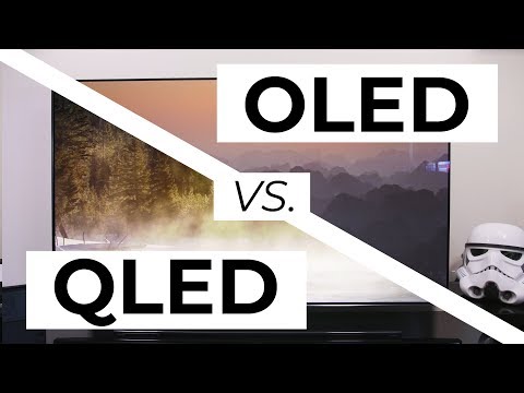
Supported by LG, Philips, Panasonic and Sony sell the OLED system TVs. OLED stands for “organic light emitting diode.” It is a fundamentally different technology from LCD, the major type of TV today. OLED is “emissive,” meaning the pixels emit their own light.
Samsung is branding its best TVs with a new acronym: “QLED” QLED (according to Samsung) stands for “quantum dot LED TV.” It is a variation of the common LED LCD, adding a quantum dot film to the LCD “sandwich.” QLED, like LCD, is, in its current form, “transmissive” and relies on an LED backlight.
OLED is the only technology capable of absolute blacks and extremely bright whites on a per-pixel basis. LCD definitely can’t do that, and even the vaunted, beloved, dearly departed plasma couldn’t do absolute blacks.
QLED, as an improvement over OLED, significantly improves the picture quality. QLED can produce an even wider range of colors than OLED, which says something about this new tech. QLED is also known to produce up to 40% higher luminance efficiency than OLED technology. Further, many tests conclude that QLED is far more efficient in terms of power consumption than its predecessor, OLED.
An exposure stop is a unit measurement of Exposure as such it provides a universal linear scale to measure the increase and decrease in light, exposed to the image sensor, due to changes in shutter speed, iso and f-stop.
+-1 stop is a doubling or halving of the amount of light let in when taking a photo
1 EV (exposure value) is just another way to say one stop of exposure change.
Same applies to shutter speed, iso and aperture.
Doubling or halving your shutter speed produces an increase or decrease of 1 stop of exposure.
Doubling or halving your iso speed produces an increase or decrease of 1 stop of exposure.
“a simple yet effective technique to estimate lighting in a single input image. Current techniques rely heavily on HDR panorama datasets to train neural networks to regress an input with limited field-of-view to a full environment map. However, these approaches often struggle with real-world, uncontrolled settings due to the limited diversity and size of their datasets. To address this problem, we leverage diffusion models trained on billions of standard images to render a chrome ball into the input image. Despite its simplicity, this task remains challenging: the diffusion models often insert incorrect or inconsistent objects and cannot readily generate images in HDR format. Our research uncovers a surprising relationship between the appearance of chrome balls and the initial diffusion noise map, which we utilize to consistently generate high-quality chrome balls. We further fine-tune an LDR difusion model (Stable Diffusion XL) with LoRA, enabling it to perform exposure bracketing for HDR light estimation. Our method produces convincing light estimates across diverse settings and demonstrates superior generalization to in-the-wild scenarios.”
DISCLAIMER – Links and images on this website may be protected by the respective owners’ copyright. All data submitted by users through this site shall be treated as freely available to share.