


COMPOSITION
-
Mastering Camera Shots and Angles: A Guide for Filmmakers
Read more: Mastering Camera Shots and Angles: A Guide for Filmmakershttps://website.ltx.studio/blog/mastering-camera-shots-and-angles
1. Extreme Wide Shot

2. Wide Shot

3. Medium Shot

4. Close Up

5. Extreme Close Up


DESIGN


COLOR
-
sRGB vs REC709 – An introduction and FFmpeg implementations
Read more: sRGB vs REC709 – An introduction and FFmpeg implementations
1. Basic Comparison
- What they are
- sRGB: A standard “web”/computer-display RGB color space defined by IEC 61966-2-1. It’s used for most monitors, cameras, printers, and the vast majority of images on the Internet.
- Rec. 709: An HD-video color space defined by ITU-R BT.709. It’s the go-to standard for HDTV broadcasts, Blu-ray discs, and professional video pipelines.
- Why they exist
- sRGB: Ensures consistent colors across different consumer devices (PCs, phones, webcams).
- Rec. 709: Ensures consistent colors across video production and playback chains (cameras → editing → broadcast → TV).
- What you’ll see
- On your desktop or phone, images tagged sRGB will look “right” without extra tweaking.
- On an HDTV or video-editing timeline, footage tagged Rec. 709 will display accurate contrast and hue on broadcast-grade monitors.
2. Digging Deeper
Feature sRGB Rec. 709 White point D65 (6504 K), same for both D65 (6504 K) Primaries (x,y) R: (0.640, 0.330) G: (0.300, 0.600) B: (0.150, 0.060) R: (0.640, 0.330) G: (0.300, 0.600) B: (0.150, 0.060) Gamut size Identical triangle on CIE 1931 chart Identical to sRGB Gamma / transfer Piecewise curve: approximate 2.2 with linear toe Pure power-law γ≈2.4 (often approximated as 2.2 in practice) Matrix coefficients N/A (pure RGB usage) Y = 0.2126 R + 0.7152 G + 0.0722 B (Rec. 709 matrix) Typical bit-depth 8-bit/channel (with 16-bit variants) 8-bit/channel (10-bit for professional video) Usage metadata Tagged as “sRGB” in image files (PNG, JPEG, etc.) Tagged as “bt709” in video containers (MP4, MOV) Color range Full-range RGB (0–255) Studio-range Y′CbCr (Y′ [16–235], Cb/Cr [16–240])
Why the Small Differences Matter
(more…) - What they are
-
Stefan Ringelschwandtner – LUT Inspector tool
Read more: Stefan Ringelschwandtner – LUT Inspector toolIt lets you load any .cube LUT right in your browser, see the RGB curves, and use a split view on the Granger Test Image to compare the original vs. LUT-applied version in real time — perfect for spotting hue shifts, saturation changes, and contrast tweaks.
https://mononodes.com/lut-inspector/


-
The 7 key elements of brand identity design + 10 corporate identity examples
Read more: The 7 key elements of brand identity design + 10 corporate identity exampleswww.lucidpress.com/blog/the-7-key-elements-of-brand-identity-design
1. Clear brand purpose and positioning
2. Thorough market research
3. Likable brand personality
4. Memorable logo
5. Attractive color palette
6. Professional typography
7. On-brand supporting graphics


LIGHTING
-
Lighting Every Darkness with 3DGS: Fast Training and Real-Time Rendering and Denoising for HDR View Synthesis
Read more: Lighting Every Darkness with 3DGS: Fast Training and Real-Time Rendering and Denoising for HDR View Synthesishttps://srameo.github.io/projects/le3d/
LE3D is a method for real-time HDR view synthesis from RAW images. It is particularly effective for nighttime scenes.
https://github.com/Srameo/LE3D


-
Magnific.ai Relight – change the entire lighting of a scene
Read more: Magnific.ai Relight – change the entire lighting of a scene
It’s a new Magnific spell that allows you to change the entire lighting of a scene and, optionally, the background with just:
1/ A prompt OR
2/ A reference image OR
3/ A light map (drawing your own lights)https://x.com/javilopen/status/1805274155065176489


-
Capturing the world in HDR for real time projects – Call of Duty: Advanced Warfare
Read more: Capturing the world in HDR for real time projects – Call of Duty: Advanced WarfareReal-World Measurements for Call of Duty: Advanced Warfare
www.activision.com/cdn/research/Real_World_Measurements_for_Call_of_Duty_Advanced_Warfare.pdf
Local version
Real_World_Measurements_for_Call_of_Duty_Advanced_Warfare.pdf

-
Light and Matter : The 2018 theory of Physically-Based Rendering and Shading by Allegorithmic
Read more: Light and Matter : The 2018 theory of Physically-Based Rendering and Shading by Allegorithmicacademy.substance3d.com/courses/the-pbr-guide-part-1
academy.substance3d.com/courses/the-pbr-guide-part-2

 Local copy:
-
Cinematographers Blueprint 300dpi poster
Read more: Cinematographers Blueprint 300dpi posterThe 300dpi digital poster is now available to all PixelSham.com subscribers.

If you have already subscribed and wish a copy, please send me a note through the contact page.
-
RawTherapee – a free, open source, cross-platform raw image and HDRi processing program
Read more: RawTherapee – a free, open source, cross-platform raw image and HDRi processing program5.10 of this tool includes excellent tools to clean up cr2 and cr3 used on set to support HDRI processing.
Converting raw to AcesCG 32 bit tiffs with metadata.


-
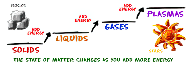
How are Energy and Matter the Same?
Read more: How are Energy and Matter the Same?www.turnerpublishing.com/blog/detail/everything-is-energy-everything-is-one-everything-is-possible/
www.universetoday.com/116615/how-are-energy-and-matter-the-same/
As Einstein showed us, light and matter and just aspects of the same thing. Matter is just frozen light. And light is matter on the move. Albert Einstein’s most famous equation says that energy and matter are two sides of the same coin. How does one become the other?
Relativity requires that the faster an object moves, the more mass it appears to have. This means that somehow part of the energy of the car’s motion appears to transform into mass. Hence the origin of Einstein’s equation. How does that happen? We don’t really know. We only know that it does.
Matter is 99.999999999999 percent empty space. Not only do the atom and solid matter consist mainly of empty space, it is the same in outer space
The quantum theory researchers discovered the answer: Not only do particles consist of energy, but so does the space between. This is the so-called zero-point energy. Therefore it is true: Everything consists of energy.
Energy is the basis of material reality. Every type of particle is conceived of as a quantum vibration in a field: Electrons are vibrations in electron fields, protons vibrate in a proton field, and so on. Everything is energy, and everything is connected to everything else through fields.


COLLECTIONS
| Featured AI
| Design And Composition
| Explore posts
POPULAR SEARCHES
unreal | pipeline | virtual production | free | learn | photoshop | 360 | macro | google | nvidia | resolution | open source | hdri | real-time | photography basics | nuke
FEATURED POSTS
-
Decart AI Mirage – The first ever World Transformation Model – turning any video, game, or camera feed into a new digital world, in real time
-
How do LLMs like ChatGPT (Generative Pre-Trained Transformer) work? Explained by Deep-Fake Ryan Gosling
-
WhatDreamsCost Spline-Path-Control – Create motion controls for ComfyUI
-
sRGB vs REC709 – An introduction and FFmpeg implementations
-
Game Development tips
-
GretagMacbeth Color Checker Numeric Values and Middle Gray
-
Cinematographers Blueprint 300dpi poster
-
Ethan Roffler interviews CG Supervisor Daniele Tosti
Social Links
DISCLAIMER – Links and images on this website may be protected by the respective owners’ copyright. All data submitted by users through this site shall be treated as freely available to share.
