slowmoVideo is an OpenSource program that creates slow-motion videos from your footage.
Slow motion cinematography is the result of playing back frames for a longer duration than they were exposed. For example, if you expose 240 frames of film in one second, then play them back at 24 fps, the resulting movie is 10 times longer (slower) than the original filmed event….
Film cameras are relatively simple mechanical devices that allow you to crank up the speed to whatever rate the shutter and pull-down mechanism allow. Some film cameras can operate at 2,500 fps or higher (although film shot in these cameras often needs some readjustment in postproduction). Video, on the other hand, is always captured, recorded, and played back at a fixed rate, with a current limit around 60fps. This makes extreme slow motion effects harder to achieve (and less elegant) on video, because slowing down the video results in each frame held still on the screen for a long time, whereas with high-frame-rate film there are plenty of frames to fill the longer durations of time. On video, the slow motion effect is more like a slide show than smooth, continuous motion.
One obvious solution is to shoot film at high speed, then transfer it to video (a case where film still has a clear advantage, sorry George). Another possibility is to cross dissolve or blur from one frame to the next. This adds a smooth transition from one still frame to the next. The blur reduces the sharpness of the image, and compared to slowing down images shot at a high frame rate, this is somewhat of a cheat. However, there isn’t much you can do about it until video can be recorded at much higher rates. Of course, many film cameras can’t shoot at high frame rates either, so the whole super-slow-motion endeavor is somewhat specialized no matter what medium you are using. (There are some high speed digital cameras available now that allow you to capture lots of digital frames directly to your computer, so technology is starting to catch up with film. However, this feature isn’t going to appear in consumer camcorders any time soon.)
this is the epic story of a group of talented digital artists trying to overcame daily technical challenges to achieve incredibly photorealistic projects of monsters and aliens
The goals of lighting in 3D computer graphics are more or less the same as those of real world lighting.
Lighting serves a basic function of bringing out, or pushing back the shapes of objects visible from the camera’s view.
It gives a two-dimensional image on the monitor an illusion of the third dimension-depth.
But it does not just stop there. It gives an image its personality, its character. A scene lit in different ways can give a feeling of happiness, of sorrow, of fear etc., and it can do so in dramatic or subtle ways. Along with personality and character, lighting fills a scene with emotion that is directly transmitted to the viewer.
Trying to simulate a real environment in an artificial one can be a daunting task. But even if you make your 3D rendering look absolutely photo-realistic, it doesn’t guarantee that the image carries enough emotion to elicit a “wow” from the people viewing it.
Making 3D renderings photo-realistic can be hard. Putting deep emotions in them can be even harder. However, if you plan out your lighting strategy for the mood and emotion that you want your rendering to express, you make the process easier for yourself.
Each light source can be broken down in to 4 distinct components and analyzed accordingly.
· Intensity
· Direction
· Color
· Size
The overall thrust of this writing is to produce photo-realistic images by applying good lighting techniques.
In the retina, photoreceptors, bipolar cells, and horizontal cells work together to process visual information before it reaches the brain. Here’s how each cell type contributes to vision:
Answering the question that is often asked, “Do I need to use ACEScg to display an sRGB monitor in the end?” (Demonstration shown at an in-house seminar) Comparison of scanlineRender output with extreme color lights on color charts with sRGB/ACREScg in color – OCIO -working space in Nuke
One problem with sRGB is that in a gradient between blue and white, it becomes a bit purple in the middle of the transition. That’s because sRGB really isn’t created to mimic how the eye sees colors; rather, it is based on how CRT monitors work. That means it works with certain frequencies of red, green, and blue, and also the non-linear coding called gamma. It’s a miracle it works as well as it does, but it’s not connected to color perception. When using those tools, you sometimes get surprising results, like purple in the gradient.
There were also attempts to create simple models matching human perception based on XYZ, but as it turned out, it’s not possible to model all color vision that way. Perception of color is incredibly complex and depends, among other things, on whether it is dark or light in the room and the background color it is against. When you look at a photograph, it also depends on what you think the color of the light source is. The dress is a typical example of color vision being very context-dependent. It is almost impossible to model this perfectly.
I based Oklab on two other color spaces, CIECAM16 and IPT. I used the lightness and saturation prediction from CIECAM16, which is a color appearance model, as a target. I actually wanted to use the datasets used to create CIECAM16, but I couldn’t find them.
IPT was designed to have better hue uniformity. In experiments, they asked people to match light and dark colors, saturated and unsaturated colors, which resulted in a dataset for which colors, subjectively, have the same hue. IPT has a few other issues but is the basis for hue in Oklab.
In the Munsell color system, colors are described with three parameters, designed to match the perceived appearance of colors: Hue, Chroma and Value. The parameters are designed to be independent and each have a uniform scale. This results in a color solid with an irregular shape. The parameters are designed to be independent and each have a uniform scale. This results in a color solid with an irregular shape. Modern color spaces and models, such as CIELAB, Cam16 and Björn Ottosson own Oklab, are very similar in their construction.
By far the most used color spaces today for color picking are HSL and HSV, two representations introduced in the classic 1978 paper “Color Spaces for Computer Graphics”. HSL and HSV designed to roughly correlate with perceptual color properties while being very simple and cheap to compute.
Today HSL and HSV are most commonly used together with the sRGB color space.
One of the main advantages of HSL and HSV over the different Lab color spaces is that they map the sRGB gamut to a cylinder. This makes them easy to use since all parameters can be changed independently, without the risk of creating colors outside of the target gamut.
The main drawback on the other hand is that their properties don’t match human perception particularly well.
Reconciling these conflicting goals perfectly isn’t possible, but given that HSV and HSL don’t use anything derived from experiments relating to human perception, creating something that makes a better tradeoff does not seem unreasonable.
With this new lightness estimate, we are ready to look into the construction of Okhsv and Okhsl.
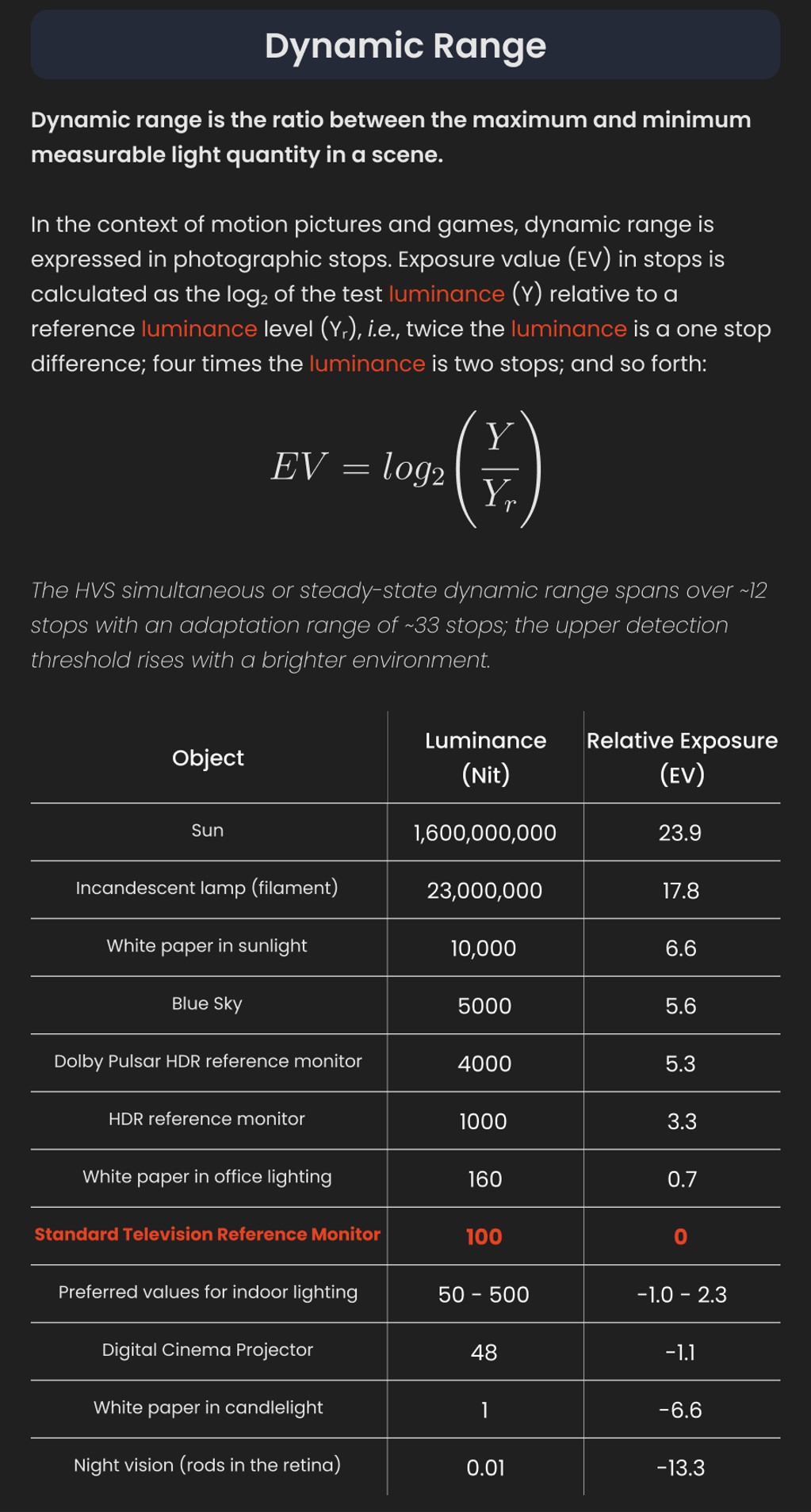
In photography, exposure value (EV) is a number that represents a combination of a camera’s shutter speed and f-number, such that all combinations that yield the same exposure have the same EV (for any fixed scene luminance).
The EV concept was developed in an attempt to simplify choosing among combinations of equivalent camera settings. Although all camera settings with the same EV nominally give the same exposure, they do not necessarily give the same picture. EV is also used to indicate an interval on the photographic exposure scale. 1 EV corresponding to a standard power-of-2 exposure step, commonly referred to as a stop
EV 0 corresponds to an exposure time of 1 sec and a relative aperture of f/1.0. If the EV is known, it can be used to select combinations of exposure time and f-number.
Note EV does not equal to photographic exposure. Photographic Exposureis defined as how much light hits the camera’s sensor. It depends on the camera settings mainly aperture and shutter speed. Exposure value (known as EV) is a number that represents theexposure setting of the camera.
Thus, strictly, EV is not a measure of luminance (indirect or reflected exposure) or illuminance (incidentl exposure); rather, an EV corresponds to a luminance (or illuminance) for which a camera with a given ISO speed would use the indicated EV to obtain the nominally correct exposure. Nonetheless, it is common practice among photographic equipment manufacturers to express luminance in EV for ISO 100 speed, as when specifying metering range or autofocus sensitivity.
The exposure depends on two things: how much light gets through the lenses to the camera’s sensor and for how long the sensor is exposed. The former is a function of the aperture value while the latter is a function of the shutter speed. Exposure value is a number that represents this potential amount of light that could hit the sensor. It is important to understand that exposure value is a measure of how exposed the sensor is to light and not a measure of how much light actually hits the sensor. The exposure value is independent of how lit the scene is. For example a pair of aperture value and shutter speed represents the same exposure value both if the camera is used during a very bright day or during a dark night.
Each exposure value number represents all the possible shutter and aperture settings that result in the same exposure. Although the exposure value is the same for different combinations of aperture values and shutter speeds the resulting photo can be very different (the aperture controls the depth of field while shutter speed controls how much motion is captured).
EV 0.0 is defined as the exposure when setting the aperture to f-number 1.0 and the shutter speed to 1 second. All other exposure values are relative to that number. Exposure values are on a base two logarithmic scale. This means that every single step of EV – plus or minus 1 – represents the exposure (actual light that hits the sensor) being halved or doubled.
5.10 of this tool includes excellent tools to clean up cr2 and cr3 used on set to support HDRI processing.
Converting raw to AcesCG 32 bit tiffs with metadata.
Divesh Naidoo: The video below was made with a live in-camera preview and auto-exposure matching, no camera solve, no HDRI capture and no manual compositing setup. Using the new Simulon phone app.
IES profiles are useful for creating life-like lighting, as they can represent the physical distribution of light from any light source.
The IES format was created by the Illumination Engineering Society, and most lighting manufacturers provide IES profile for the lights they manufacture.
DISCLAIMER – Links and images on this website may be protected by the respective owners’ copyright. All data submitted by users through this site shall be treated as freely available to share.