ACES 2.0 is the second major release of the components that make up the ACES system. The most significant change is a new suite of rendering transforms whose design was informed by collected feedback and requests from users of ACES 1. The changes aim to improve the appearance of perceived artifacts and to complete previously unfinished components of the system, resulting in a more complete, robust, and consistent product.
Highlights of the key changes in ACES 2.0 are as follows:
New output transforms, including:
A less aggressive tone scale
More intuitive controls to create custom outputs to non-standard displays
Robust gamut mapping to improve perceptual uniformity
Improved performance of the inverse transforms
Enhanced AMF specification
An updated specification for ACES Transform IDs
OpenEXR compression recommendations
Enhanced tools for generating Input Transforms and recommended procedures for characterizing prosumer cameras
Look Transform Library
Expanded documentation
Rendering Transform
The most substantial change in ACES 2.0 is a complete redesign of the rendering transform.
ACES 2.0 was built as a unified system, rather than through piecemeal additions. Different deliverable outputs “match” better and making outputs to display setups other than the provided presets is intended to be user-driven. The rendering transforms are less likely to produce undesirable artifacts “out of the box”, which means less time can be spent fixing problematic images and more time making pictures look the way you want.
Key design goals
Improve consistency of tone scale and provide an easy to use parameter to allow for outputs between preset dynamic ranges
Minimize hue skews across exposure range in a region of same hue
Unify for structural consistency across transform type
Easy to use parameters to create outputs other than the presets
Robust gamut mapping to improve harsh clipping artifacts
Fill extents of output code value cube (where appropriate and expected)
Invertible – not necessarily reversible, but Output > ACES > Output round-trip should be possible
Accomplish all of the above while maintaining an acceptable “out-of-the box” rendering
“Fix your gaze on the black dot on the left side of this image. But wait! Finish reading this paragraph first. As you gaze at the left dot, try to answer this question: In what direction is the object on the right moving? Is it drifting diagonally, or is it moving up and down?”
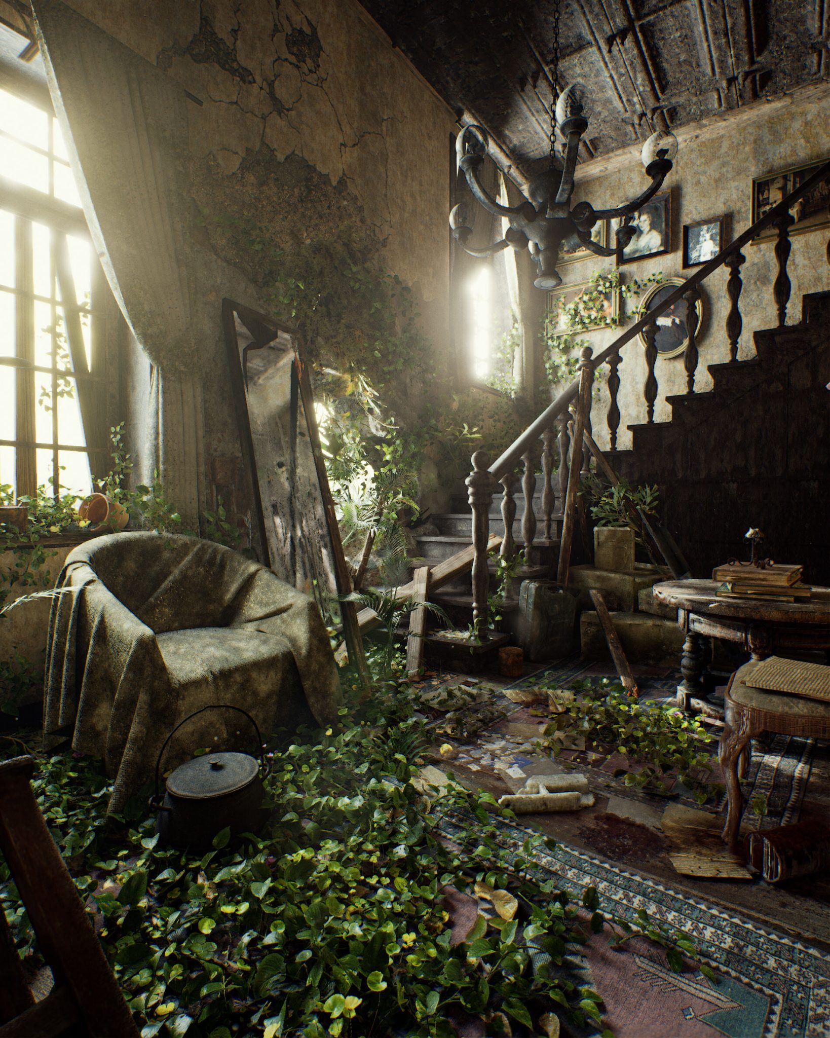
Answering the question that is often asked, “Do I need to use ACEScg to display an sRGB monitor in the end?” (Demonstration shown at an in-house seminar) Comparison of scanlineRender output with extreme color lights on color charts with sRGB/ACREScg in color – OCIO -working space in Nuke
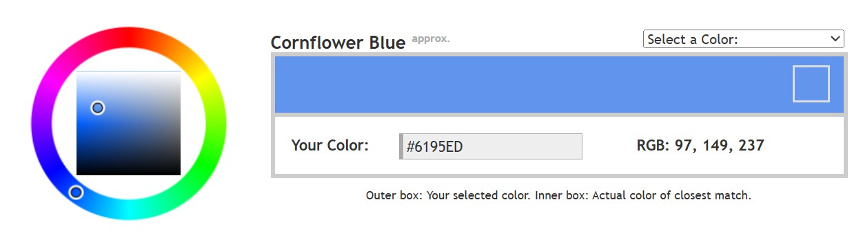
The way humans see the world… until we have a way to describe something, even something so fundamental as a colour, we may not even notice that something it’s there.
Ancient languages didn’t have a word for blue — not Greek, not Chinese, not Japanese, not Hebrew, not Icelandic cultures. And without a word for the colour, there’s evidence that they may not have seen it at all. https://www.wnycstudios.org/story/211119-colors
Every language first had a word for black and for white, or dark and light. The next word for a colour to come into existence — in every language studied around the world — was red, the colour of blood and wine. After red, historically, yellow appears, and later, green (though in a couple of languages, yellow and green switch places). The last of these colours to appear in every language is blue.
The only ancient culture to develop a word for blue was the Egyptians — and as it happens, they were also the only culture that had a way to produce a blue dye. https://mymodernmet.com/shades-of-blue-color-history/
True blue hues are rare in the natural world because synthesizing pigments that absorb longer-wavelength light (reds and yellows) while reflecting shorter-wavelength blue light requires exceptionally elaborate molecular structures—biochemical feats that most plants and animals simply don’t undertake.
When you gaze at a blueberry’s deep blue surface, you’re actually seeing structural coloration rather than a true blue pigment. A fine, waxy bloom on the berry’s skin contains nanostructures that preferentially scatter blue and violet light, giving the fruit its signature blue sheen even though its inherent pigment is reddish.
Similarly, many of nature’s most striking blues—like those of blue jays and morpho butterflies—arise not from blue pigments but from microscopic architectures in feathers or wing scales. These tiny ridges and air pockets manipulate incoming light so that blue wavelengths emerge most prominently, creating vivid, angle-dependent colors through scattering rather than pigment alone.
In the retina, photoreceptors, bipolar cells, and horizontal cells work together to process visual information before it reaches the brain. Here’s how each cell type contributes to vision:
Black-body radiation is the type of electromagnetic radiation within or surrounding a body in thermodynamic equilibrium with its environment, or emitted by a black body (an opaque and non-reflective body) held at constant, uniform temperature. The radiation has a specific spectrum and intensity that depends only on the temperature of the body.
A black-body at room temperature appears black, as most of the energy it radiates is infra-red and cannot be perceived by the human eye. At higher temperatures, black bodies glow with increasing intensity and colors that range from dull red to blindingly brilliant blue-white as the temperature increases.
import math,sys

def Exposure2Intensity(exposure):
    exp = float(exposure)
    result = math.pow(2,exp)
    print(result)

Exposure2Intensity(0)

def Intensity2Exposure(intensity):
    inarg = float(intensity)

    if inarg == 0:
        print("Exposure of zero intensity is undefined.")
        return

    if inarg < 1e-323:
        inarg = max(inarg, 1e-323)
        print("Exposure of negative intensities is undefined. Clamping to a very small value instead (1e-323)")

    result = math.log(inarg, 2)
    print(result)

Intensity2Exposure(0.1)
Why Exposure?
Exposure is a stop value that multiplies the intensity by 2 to the power of the stop. Increasing exposure by 1 results in double the amount of light.
Artists think in “stops.” Doubling or halving brightness is easy math and common in grading and look-dev. Exposure counts doublings in whole stops:
+1 stop = ×2 brightness
−1 stop = ×0.5 brightness
This gives perceptually even controls across both bright and dark values.
Why Intensity?
Intensity is linear. It’s what render engines and compositors expect when:
Summing values
Averaging pixels
Multiplying or filtering pixel data
Use intensity when you need the actual math on pixel/light data.
Formulas (from your Python)
Intensity from exposure: intensity = 2**exposure
Exposure from intensity: exposure = log₂(intensity)
Guardrails:
Intensity must be > 0 to compute exposure.
If intensity = 0 → exposure is undefined.
Clamp tiny values (e.g. 1e−323) before using log₂.
Use Exposure (stops) when…
You want artist-friendly sliders (−5…+5 stops)
Adjusting look-dev or grading in even stops
Matching plates with quick ±1 stop tweaks
Tweening brightness changes smoothly across ranges
Use Intensity (linear) when…
Storing raw pixel/light values
Multiplying textures or lights by a gain
Performing sums, averages, and filters
Feeding values to render engines expecting linear data
Examples
+2 stops → 2**2 = 4.0 (×4)
+1 stop → 2**1 = 2.0 (×2)
0 stop → 2**0 = 1.0 (×1)
−1 stop → 2**(−1) = 0.5 (×0.5)
−2 stops → 2**(−2) = 0.25 (×0.25)
Intensity 0.1 → exposure = log₂(0.1) ≈ −3.32
Rule of thumb
Think in stops (exposure) for controls and matching. Compute in linear (intensity) for rendering and math.
This 2025 I decided to start learning how to code, so I installed Visual Studio and I started looking into C++. After days of watching tutorials and guides about the basics of C++ and programming, I decided to make something physics-related. I started with a dot that fell to the ground and then I wanted to simulate gravitational attraction, so I made 2 circles attracting each other. I thought it was really cool to see something I made with code actually work, so I kept building on top of that small, basic program. And here we are after roughly 8 months of learning programming. This is Galaxy Engine, and it is a simulation software I have been making ever since I started my learning journey. It currently can simulate gravity, dark matter, galaxies, the Big Bang, temperature, fluid dynamics, breakable solids, planetary interactions, etc. The program can run many tens of thousands of particles in real time on the CPU thanks to the Barnes-Hut algorithm, mixed with Morton curves. It also includes its own PBR 2D path tracer with BVH optimizations. The path tracer can simulate a bunch of stuff like diffuse lighting, specular reflections, refraction, internal reflection, fresnel, emission, dispersion, roughness, IOR, nested IOR and more! I tried to make the path tracer closer to traditional 3D render engines like V-Ray. I honestly never imagined I would go this far with programming, and it has been an amazing learning experience so far. I think that mixing this knowledge with my 3D knowledge can unlock countless new possibilities. In case you are curious about Galaxy Engine, I made it completely free and Open-Source so that anyone can build and compile it locally! You can find the source code inGitHub
A way to approximate complex lighting in ultra realistic renders.
All SH lighting techniques involve replacing parts of standard lighting equations with spherical functions that have been projected into frequency space using the spherical harmonics as a basis.
IES profiles are useful for creating life-like lighting, as they can represent the physical distribution of light from any light source.
The IES format was created by the Illumination Engineering Society, and most lighting manufacturers provide IES profile for the lights they manufacture.
DISCLAIMER – Links and images on this website may be protected by the respective owners’ copyright. All data submitted by users through this site shall be treated as freely available to share.


