A number of problems in computer vision and related fields would be mitigated if camera spectral sensitivities were known. As consumer cameras are not designed for high-precision visual tasks, manufacturers do not disclose spectral sensitivities. Their estimation requires a costly optical setup, which triggered researchers to come up with numerous indirect methods that aim to lower cost and complexity by using color targets. However, the use of color targets gives rise to new complications that make the estimation more difficult, and consequently, there currently exists no simple, low-cost, robust go-to method for spectral sensitivity estimation that non-specialized research labs can adopt. Furthermore, even if not limited by hardware or cost, researchers frequently work with imagery from multiple cameras that they do not have in their possession.
To provide a practical solution to this problem, we propose a framework for spectral sensitivity estimation that not only does not require any hardware (including a color target), but also does not require physical access to the camera itself. Similar to other work, we formulate an optimization problem that minimizes a two-term objective function: a camera-specific term from a system of equations, and a universal term that bounds the solution space.
Different than other work, we utilize publicly available high-quality calibration data to construct both terms. We use the colorimetric mapping matrices provided by the Adobe DNG Converter to formulate the camera-specific system of equations, and constrain the solutions using an autoencoder trained on a database of ground-truth curves. On average, we achieve reconstruction errors as low as those that can arise due to manufacturing imperfections between two copies of the same camera. We provide predicted sensitivities for more than 1,000 cameras that the Adobe DNG Converter currently supports, and discuss which tasks can become trivial when camera responses are available.
“The list should be helpful for every material artist who work on PBR materials as it contains over 200 color values measured with PCE-RGB2 1002 Color Spectrometer device and presented in linear and sRGB (2.2) gamma space.
All color values, HUE and Saturation in this list come from measurements taken with PCE-RGB2 1002 Color Spectrometer device and are presented in linear and sRGB (2.2) gamma space (more info at the end of this video) I calculated Relative Luminance and Luminance values based on captured color using my own equation which takes color based luminance perception into consideration. Bare in mind that there is no ‘one’ color per substance as nothing in nature is even 100% uniform and any value in +/-10% range from these should be considered as correct one. Therefore this list should be always considered as a color reference for material’s albedos, not ulitimate and absolute truth.“
A LUT (Lookup Table) is essentially the modifier between two images, the original image and the displayed image, based on a mathematical formula. Basically conversion matrices of different complexities. There are different types of LUTS – viewing, transform, calibration, 1D and 3D.
Of all the pigments that have been banned over the centuries, the color most missed by painters is likely Lead White.
This hue could capture and reflect a gleam of light like no other, though its production was anything but glamorous. The 17th-century Dutch method for manufacturing the pigment involved layering cow and horse manure over lead and vinegar. After three months in a sealed room, these materials would combine to create flakes of pure white. While scientists in the late 19th century identified lead as poisonous, it wasn’t until 1978 that the United States banned the production of lead white paint.
Most software around us today are decent at accurately displaying colors. Processing of colors is another story unfortunately, and is often done badly.
To understand what the problem is, let’s start with an example of three ways of blending green and magenta:
Perceptual blend – A smooth transition using a model designed to mimic human perception of color. The blending is done so that the perceived brightness and color varies smoothly and evenly.
Linear blend – A model for blending color based on how light behaves physically. This type of blending can occur in many ways naturally, for example when colors are blended together by focus blur in a camera or when viewing a pattern of two colors at a distance.
sRGB blend – This is how colors would normally be blended in computer software, using sRGB to represent the colors.
Let’s look at some more examples of blending of colors, to see how these problems surface more practically. The examples use strong colors since then the differences are more pronounced. This is using the same three ways of blending colors as the first example.
Instead of making it as easy as possible to work with color, most software make it unnecessarily hard, by doing image processing with representations not designed for it. Approximating the physical behavior of light with linear RGB models is one easy thing to do, but more work is needed to create image representations tailored for image processing and human perception.
import math,sys

def Exposure2Intensity(exposure):
    exp = float(exposure)
    result = math.pow(2,exp)
    print(result)

Exposure2Intensity(0)

def Intensity2Exposure(intensity):
    inarg = float(intensity)

    if inarg == 0:
        print("Exposure of zero intensity is undefined.")
        return

    if inarg < 1e-323:
        inarg = max(inarg, 1e-323)
        print("Exposure of negative intensities is undefined. Clamping to a very small value instead (1e-323)")

    result = math.log(inarg, 2)
    print(result)

Intensity2Exposure(0.1)
Why Exposure?
Exposure is a stop value that multiplies the intensity by 2 to the power of the stop. Increasing exposure by 1 results in double the amount of light.
Artists think in “stops.” Doubling or halving brightness is easy math and common in grading and look-dev. Exposure counts doublings in whole stops:
+1 stop = ×2 brightness
−1 stop = ×0.5 brightness
This gives perceptually even controls across both bright and dark values.
Why Intensity?
Intensity is linear. It’s what render engines and compositors expect when:
Summing values
Averaging pixels
Multiplying or filtering pixel data
Use intensity when you need the actual math on pixel/light data.
Formulas (from your Python)
Intensity from exposure: intensity = 2**exposure
Exposure from intensity: exposure = log₂(intensity)
Guardrails:
Intensity must be > 0 to compute exposure.
If intensity = 0 → exposure is undefined.
Clamp tiny values (e.g. 1e−323) before using log₂.
Use Exposure (stops) when…
You want artist-friendly sliders (−5…+5 stops)
Adjusting look-dev or grading in even stops
Matching plates with quick ±1 stop tweaks
Tweening brightness changes smoothly across ranges
Use Intensity (linear) when…
Storing raw pixel/light values
Multiplying textures or lights by a gain
Performing sums, averages, and filters
Feeding values to render engines expecting linear data
Examples
+2 stops → 2**2 = 4.0 (×4)
+1 stop → 2**1 = 2.0 (×2)
0 stop → 2**0 = 1.0 (×1)
−1 stop → 2**(−1) = 0.5 (×0.5)
−2 stops → 2**(−2) = 0.25 (×0.25)
Intensity 0.1 → exposure = log₂(0.1) ≈ −3.32
Rule of thumb
Think in stops (exposure) for controls and matching. Compute in linear (intensity) for rendering and math.
When collecting hdri make sure the data supports basic metadata, such as:
Iso
Aperture
Exposure time or shutter time
Color temperature
Color space Exposure value (what the sensor receives of the sun intensity in lux)
7+ brackets (with 5 or 6 being the perceived balanced exposure)
In image processing, computer graphics, and photography, high dynamic range imaging (HDRI or just HDR) is a set of techniques that allow a greater dynamic range of luminances (a Photometry measure of the luminous intensity per unit area of light travelling in a given direction. It describes the amount of light that passes through or is emitted from a particular area, and falls within a given solid angle) between the lightest and darkest areas of an image than standard digital imaging techniques or photographic methods. This wider dynamic range allows HDR images to represent more accurately the wide range of intensity levels found in real scenes ranging from direct sunlight to faint starlight and to the deepest shadows.
The two main sources of HDR imagery are computer renderings and merging of multiple photographs, which in turn are known as low dynamic range (LDR) or standard dynamic range (SDR) images. Tone Mapping (Look-up) techniques, which reduce overall contrast to facilitate display of HDR images on devices with lower dynamic range, can be applied to produce images with preserved or exaggerated local contrast for artistic effect. Photography
In photography, dynamic range is measured in Exposure Values (in photography, exposure value denotes all combinations of camera shutter speed and relative aperture that give the same exposure. The concept was developed in Germany in the 1950s) differences or stops, between the brightest and darkest parts of the image that show detail. An increase of one EV or one stop is a doubling of the amount of light.
The human response to brightness is well approximated by a Steven’s power law, which over a reasonable range is close to logarithmic, as described by the Weber�Fechner law, which is one reason that logarithmic measures of light intensity are often used as well.
HDR is short for High Dynamic Range. It’s a term used to describe an image which contains a greater exposure range than the “black” to “white” that 8 or 16-bit integer formats (JPEG, TIFF, PNG) can describe. Whereas these Low Dynamic Range images (LDR) can hold perhaps 8 to 10 f-stops of image information, HDR images can describe beyond 30 stops and stored in 32 bit images.
In the retina, photoreceptors, bipolar cells, and horizontal cells work together to process visual information before it reaches the brain. Here’s how each cell type contributes to vision:
DISCLAIMER – Links and images on this website may be protected by the respective owners’ copyright. All data submitted by users through this site shall be treated as freely available to share.


 Local copy:


