import math,sys

def Exposure2Intensity(exposure):
    exp = float(exposure)
    result = math.pow(2,exp)
    print(result)

Exposure2Intensity(0)

def Intensity2Exposure(intensity):
    inarg = float(intensity)

    if inarg == 0:
        print("Exposure of zero intensity is undefined.")
        return

    if inarg < 1e-323:
        inarg = max(inarg, 1e-323)
        print("Exposure of negative intensities is undefined. Clamping to a very small value instead (1e-323)")

    result = math.log(inarg, 2)
    print(result)

Intensity2Exposure(0.1)
Why Exposure?
Exposure is a stop value that multiplies the intensity by 2 to the power of the stop. Increasing exposure by 1 results in double the amount of light.
Artists think in “stops.” Doubling or halving brightness is easy math and common in grading and look-dev. Exposure counts doublings in whole stops:
+1 stop = ×2 brightness
−1 stop = ×0.5 brightness
This gives perceptually even controls across both bright and dark values.
Why Intensity?
Intensity is linear. It’s what render engines and compositors expect when:
Summing values
Averaging pixels
Multiplying or filtering pixel data
Use intensity when you need the actual math on pixel/light data.
Formulas (from your Python)
Intensity from exposure: intensity = 2**exposure
Exposure from intensity: exposure = log₂(intensity)
Guardrails:
Intensity must be > 0 to compute exposure.
If intensity = 0 → exposure is undefined.
Clamp tiny values (e.g. 1e−323) before using log₂.
Use Exposure (stops) when…
You want artist-friendly sliders (−5…+5 stops)
Adjusting look-dev or grading in even stops
Matching plates with quick ±1 stop tweaks
Tweening brightness changes smoothly across ranges
Use Intensity (linear) when…
Storing raw pixel/light values
Multiplying textures or lights by a gain
Performing sums, averages, and filters
Feeding values to render engines expecting linear data
Examples
+2 stops → 2**2 = 4.0 (×4)
+1 stop → 2**1 = 2.0 (×2)
0 stop → 2**0 = 1.0 (×1)
−1 stop → 2**(−1) = 0.5 (×0.5)
−2 stops → 2**(−2) = 0.25 (×0.25)
Intensity 0.1 → exposure = log₂(0.1) ≈ −3.32
Rule of thumb
Think in stops (exposure) for controls and matching. Compute in linear (intensity) for rendering and math.
An exposure stop is a unit measurement of Exposure as such it provides a universal linear scale to measure the increase and decrease in light, exposed to the image sensor, due to changes in shutter speed, iso and f-stop.
+-1 stop is a doubling or halving of the amount of light let in when taking a photo
1 EV (exposure value) is just another way to say one stop of exposure change.
Same applies to shutter speed, iso and aperture.
Doubling or halving your shutter speed produces an increase or decrease of 1 stop of exposure.
Doubling or halving your iso speed produces an increase or decrease of 1 stop of exposure.
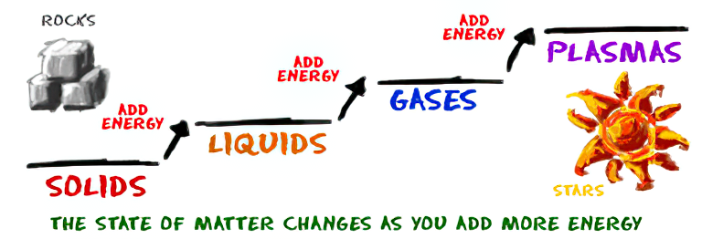
As Einstein showed us, light and matter and just aspects of the same thing. Matter is just frozen light. And light is matter on the move. Albert Einstein’s most famous equation says that energy and matter are two sides of the same coin. How does one become the other?
Relativity requires that the faster an object moves, the more mass it appears to have. This means that somehow part of the energy of the car’s motion appears to transform into mass. Hence the origin of Einstein’s equation. How does that happen? We don’t really know. We only know that it does.
Matter is 99.999999999999 percent empty space. Not only do the atom and solid matter consist mainly of empty space, it is the same in outer space
The quantum theory researchers discovered the answer: Not only do particles consist of energy, but so does the space between. This is the so-called zero-point energy. Therefore it is true: Everything consists of energy.
Energy is the basis of material reality. Every type of particle is conceived of as a quantum vibration in a field: Electrons are vibrations in electron fields, protons vibrate in a proton field, and so on. Everything is energy, and everything is connected to everything else through fields.
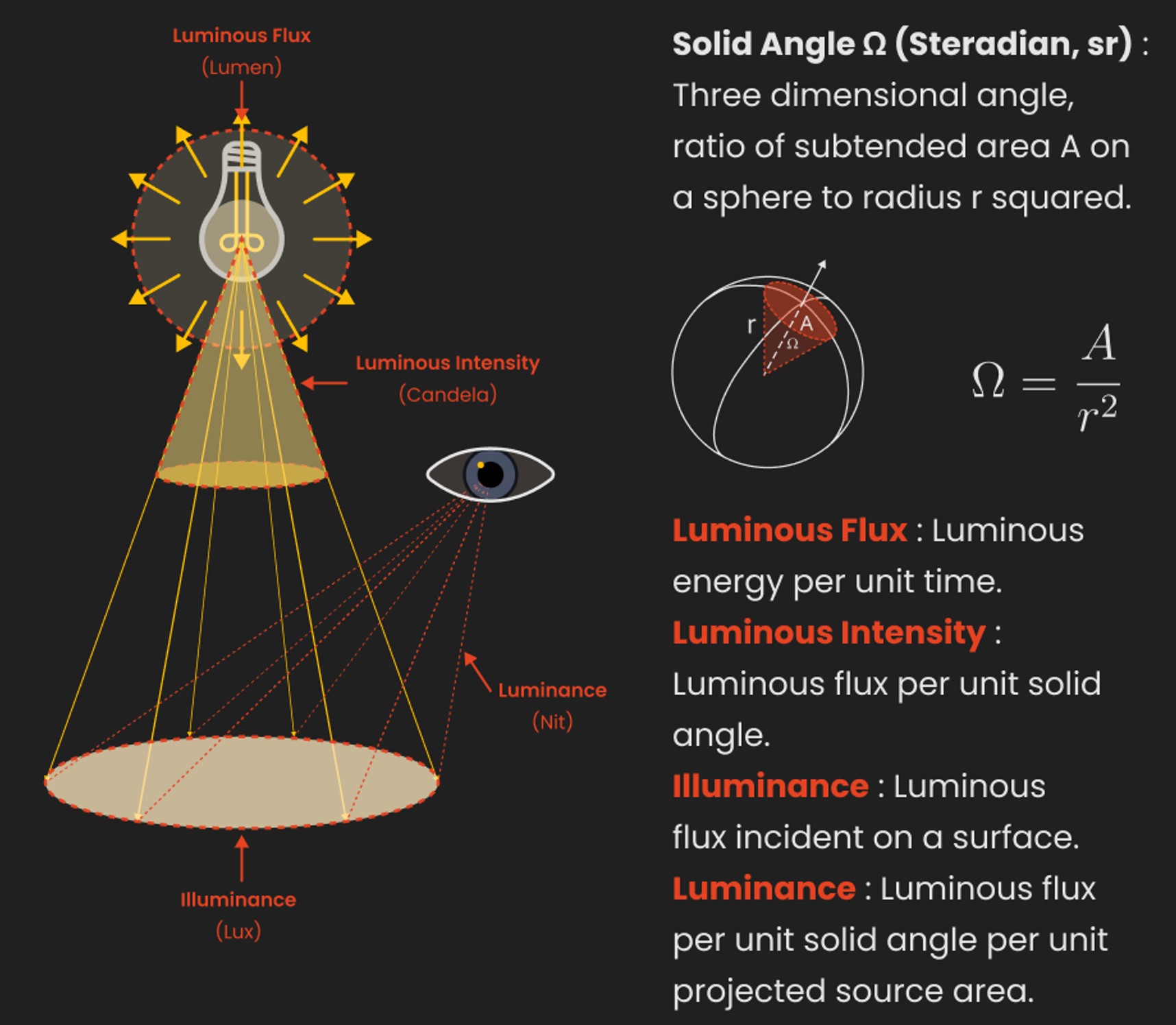
Candela is the basic unit of measure of the entire volume of light intensity from any point in a single direction from a light source. Note the detail: it measures the total volume of light within a certain beam angle and direction.
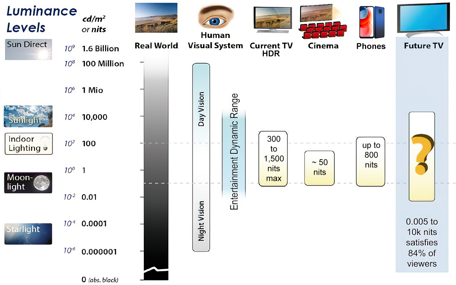
While the luminance of starlight is around 0.001 cd/m2, that of a sunlit scene is around 100,000 cd/m2, which is a hundred millions times higher. The luminance of the sun itself is approximately 1,000,000,000 cd/m2.
The candela per square metre (symbol: cd/m2) is the unit of luminance in the International System of Units (SI). The unit is based on the candela, the SI unit of luminous intensity, and the square metre, the SI unit of area. The nit (symbol: nt) is a non-SI name also used for this unit (1 nt = 1 cd/m2).[1] The term nit is believed to come from the Latin word nitēre, “to shine”. As a measure of light emitted per unit area, this unit is frequently used to specify the brightness of a display device.
NIT and cd/m2 (candela power) represent the same thing and can be used interchangeably. One nit is equivalent to one candela per square meter, where the candela is the amount of light which has been emitted by a common tallow candle, but NIT is not part of the International System of Units (abbreviated SI, from Systeme International, in French).
It’s easiest to think of a TV as emitting light directly, in much the same way as the Sun does. Nits are simply the measurement of the level of light (luminance) in a given area which the emitting source sends to your eyes or a camera sensor.
The Nit can be considered a unit of visible-light intensity which is often used to specify the brightness level of an LCD.
1 Nit is approximately equal to 3.426 Lumens. To work out a comparable number of Nits to Lumens, you need to multiply the number of Nits by 3.426. If you know the number of Lumens, and wish to know the Nits, simply divide the number of Lumens by 3.426.
Most consumer desktop LCDs have Nits of 200 to 300, the average TV most likely has an output capability of between 100 and 200 Nits, and an HDR TV ranges from 400 to 1,500 Nits.
Virtual Production sets currently sport around 6000 NIT ceiling and 1000 NIT wall panels.
The ambient brightness of a sunny day with clear blue skies is between 7000-10,000 nits (between 3000-7000 nits for overcast skies and indirect sunlight).
A bright sunny day can have specular highlights that reach over 100,000 nits. Direct sunlight is around 1,600,000,000 nits.
10,000 nits is also the typical brightness of a fluorescent tube – bright, but not painful to look at.
Tests showed that a “black level” of 0.005 nits (cd/m²) satisfied the vast majority of viewers. While 0.005 nits is very close to true black, Griffis says Dolby can go down to a black of 0.0001 nits, even though there is no need or ability for displays to get that dark today.
How bright is white? Dolby says the range of 0.005 nits – 10,000 nits satisfied 84% of the viewers in their viewing tests.
The brightest consumer HDR displays today are about 1,500 nits. Professional displays where HDR content is color-graded can achieve up to 4,000 nits peak brightness.
High brightness that would be in danger of damaging the eye would be in the neighborhood of 250,000 nits.
Lumens
Lumen is a measure of how much light is emitted (luminance, luminous flux) by an object. It indicates the total potential amount of light from a light source that is visible to the human eye.
Lumen is commonly used in the context of light bulbs or video-projectors as a metric for their brightness power.
Lumen is used to describe light output, and about video projectors, it is commonly referred to as ANSI Lumens. Simply put, lumens is how to find out how bright a LED display is. The higher the lumens, the brighter to display!
Technically speaking, a Lumen is the SI unit of luminous flux, which is equal to the amount of light which is emitted per second in a unit solid angle of one steradian from a uniform source of one-candela intensity radiating in all directions.
LUX
Lux(lx) or often Illuminance, is a photometric unit along a given area, which takes in account the sensitivity of human eye to different wavelenghts. It is the measure of light at a specific distance within a specific area at that distance. Often used to measure the incidental sun’s intensity.
DISCLAIMER – Links and images on this website may be protected by the respective owners’ copyright. All data submitted by users through this site shall be treated as freely available to share.


![[gamma correction test]](http://www.madore.org/~david/misc/color/gammatest.png "sRGB gamma correction test")