this is the epic story of a group of talented digital artists trying to overcame daily technical challenges to achieve incredibly photorealistic projects of monsters and aliens
ACES 2.0 is the second major release of the components that make up the ACES system. The most significant change is a new suite of rendering transforms whose design was informed by collected feedback and requests from users of ACES 1. The changes aim to improve the appearance of perceived artifacts and to complete previously unfinished components of the system, resulting in a more complete, robust, and consistent product.
Highlights of the key changes in ACES 2.0 are as follows:
New output transforms, including:
A less aggressive tone scale
More intuitive controls to create custom outputs to non-standard displays
Robust gamut mapping to improve perceptual uniformity
Improved performance of the inverse transforms
Enhanced AMF specification
An updated specification for ACES Transform IDs
OpenEXR compression recommendations
Enhanced tools for generating Input Transforms and recommended procedures for characterizing prosumer cameras
Look Transform Library
Expanded documentation
Rendering Transform
The most substantial change in ACES 2.0 is a complete redesign of the rendering transform.
ACES 2.0 was built as a unified system, rather than through piecemeal additions. Different deliverable outputs “match” better and making outputs to display setups other than the provided presets is intended to be user-driven. The rendering transforms are less likely to produce undesirable artifacts “out of the box”, which means less time can be spent fixing problematic images and more time making pictures look the way you want.
Key design goals
Improve consistency of tone scale and provide an easy to use parameter to allow for outputs between preset dynamic ranges
Minimize hue skews across exposure range in a region of same hue
Unify for structural consistency across transform type
Easy to use parameters to create outputs other than the presets
Robust gamut mapping to improve harsh clipping artifacts
Fill extents of output code value cube (where appropriate and expected)
Invertible – not necessarily reversible, but Output > ACES > Output round-trip should be possible
Accomplish all of the above while maintaining an acceptable “out-of-the box” rendering
Answering the question that is often asked, “Do I need to use ACEScg to display an sRGB monitor in the end?” (Demonstration shown at an in-house seminar) Comparison of scanlineRender output with extreme color lights on color charts with sRGB/ACREScg in color – OCIO -working space in Nuke
The primary goal of physically-based rendering (PBR) is to create a simulation that accurately reproduces the imaging process of electro-magnetic spectrum radiation incident to an observer. This simulation should be indistinguishable from reality for a similar observer.
Because a camera is not sensitive to incident light the same way than a human observer, the images it captures are transformed to be colorimetric. A project might require infrared imaging simulation, a portion of the electro-magnetic spectrum that is invisible to us. Radically different observers might image the same scene but the act of observing does not change the intrinsic properties of the objects being imaged. Consequently, the physical modelling of the virtual scene should be independent of the observer.
A light wave that is vibrating in more than one plane is referred to as unpolarized light. …
Polarized light waves are light waves in which the vibrations occur in a single plane. The process of transforming unpolarized light into polarized light is known as polarization.
The most common use of polarized technology is to reduce lighting complexity on the subject. Details such as glare and hard edges are not removed, but greatly reduced.
It lets you load any .cube LUT right in your browser, see the RGB curves, and use a split view on the Granger Test Image to compare the original vs. LUT-applied version in real time — perfect for spotting hue shifts, saturation changes, and contrast tweaks.
In color technology, color depth also known as bit depth, is either the number of bits used to indicate the color of a single pixel, OR the number of bits used for each color component of a single pixel.
When referring to a pixel, the concept can be defined as bits per pixel (bpp).
When referring to a color component, the concept can be defined as bits per component, bits per channel, bits per color (all three abbreviated bpc), and also bits per pixel component, bits per color channel or bits per sample (bps). Modern standards tend to use bits per component, but historical lower-depth systems used bits per pixel more often.
Color depth is only one aspect of color representation, expressing the precision with which the amount of each primary can be expressed; the other aspect is how broad a range of colors can be expressed (the gamut). The definition of both color precision and gamut is accomplished with a color encoding specification which assigns a digital code value to a location in a color space.
5.10 of this tool includes excellent tools to clean up cr2 and cr3 used on set to support HDRI processing.
Converting raw to AcesCG 32 bit tiffs with metadata.
Basically, gamma is the relationship between the brightness of a pixel as it appears on the screen, and the numerical value of that pixel. Generally Gamma is just about defining relationships.
Three main types: – Image Gamma encoded in images – Display Gammas encoded in hardware and/or viewing time – System or Viewing Gamma which is the net effect of all gammas when you look back at a final image. In theory this should flatten back to 1.0 gamma.
“The Color Rendering Index is a measurement of how faithfully a light source reveals the colors of whatever it illuminates, it describes the ability of a light source to reveal the color of an object, as compared to the color a natural light source would provide. The highest possible CRI is 100. A CRI of 100 generally refers to a perfect black body, like a tungsten light source or the sun. ”
Black-body radiation is the type of electromagnetic radiation within or surrounding a body in thermodynamic equilibrium with its environment, or emitted by a black body (an opaque and non-reflective body) held at constant, uniform temperature. The radiation has a specific spectrum and intensity that depends only on the temperature of the body.
A black-body at room temperature appears black, as most of the energy it radiates is infra-red and cannot be perceived by the human eye. At higher temperatures, black bodies glow with increasing intensity and colors that range from dull red to blindingly brilliant blue-white as the temperature increases.
Note: In Foundry’s Nuke, the software will map 18% gray to whatever your center f/stop is set to in the viewer settings (f/8 by default… change that to EV by following the instructions below).
You can experiment with this by attaching an Exposure node to a Constant set to 0.18, setting your viewer read-out to Spotmeter, and adjusting the stops in the node up and down. You will see that a full stop up or down will give you the respective next value on the aperture scale (f8, f11, f16 etc.).
One stop doubles or halves the amount or light that hits the filmback/ccd, so everything works in powers of 2.
So starting with 0.18 in your constant, you will see that raising it by a stop will give you .36 as a floating point number (in linear space), while your f/stop will be f/11 and so on.
If you set your center stop to 0 (see below) you will get a relative readout in EVs, where EV 0 again equals 18% constant gray.
In other words. Setting the center f-stop to 0 means that in a neutral plate, the middle gray in the macbeth chart will equal to exposure value 0. EV 0 corresponds to an exposure time of 1 sec and an aperture of f/1.0.
This will set the sun usually around EV12-17 and the sky EV1-4 , depending on cloud coverage.
To switch Foundry’s Nuke’s SpotMeter to return the EV of an image, click on the main viewport, and then press s, this opens the viewer’s properties. Now set the center f-stop to 0 in there. And the SpotMeter in the viewport will change from aperture and fstops to EV.
DISCLAIMER – Links and images on this website may be protected by the respective owners’ copyright. All data submitted by users through this site shall be treated as freely available to share.