


COMPOSITION
-
SlowMoVideo – How to make a slow motion shot with the open source program
Read more: SlowMoVideo – How to make a slow motion shot with the open source programhttp://slowmovideo.granjow.net/
slowmoVideo is an OpenSource program that creates slow-motion videos from your footage.
Slow motion cinematography is the result of playing back frames for a longer duration than they were exposed. For example, if you expose 240 frames of film in one second, then play them back at 24 fps, the resulting movie is 10 times longer (slower) than the original filmed event….
Film cameras are relatively simple mechanical devices that allow you to crank up the speed to whatever rate the shutter and pull-down mechanism allow. Some film cameras can operate at 2,500 fps or higher (although film shot in these cameras often needs some readjustment in postproduction). Video, on the other hand, is always captured, recorded, and played back at a fixed rate, with a current limit around 60fps. This makes extreme slow motion effects harder to achieve (and less elegant) on video, because slowing down the video results in each frame held still on the screen for a long time, whereas with high-frame-rate film there are plenty of frames to fill the longer durations of time. On video, the slow motion effect is more like a slide show than smooth, continuous motion.
One obvious solution is to shoot film at high speed, then transfer it to video (a case where film still has a clear advantage, sorry George). Another possibility is to cross dissolve or blur from one frame to the next. This adds a smooth transition from one still frame to the next. The blur reduces the sharpness of the image, and compared to slowing down images shot at a high frame rate, this is somewhat of a cheat. However, there isn’t much you can do about it until video can be recorded at much higher rates. Of course, many film cameras can’t shoot at high frame rates either, so the whole super-slow-motion endeavor is somewhat specialized no matter what medium you are using. (There are some high speed digital cameras available now that allow you to capture lots of digital frames directly to your computer, so technology is starting to catch up with film. However, this feature isn’t going to appear in consumer camcorders any time soon.)


DESIGN
-
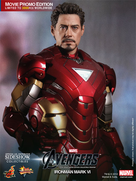
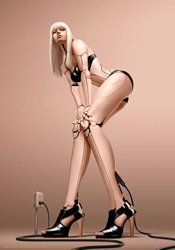
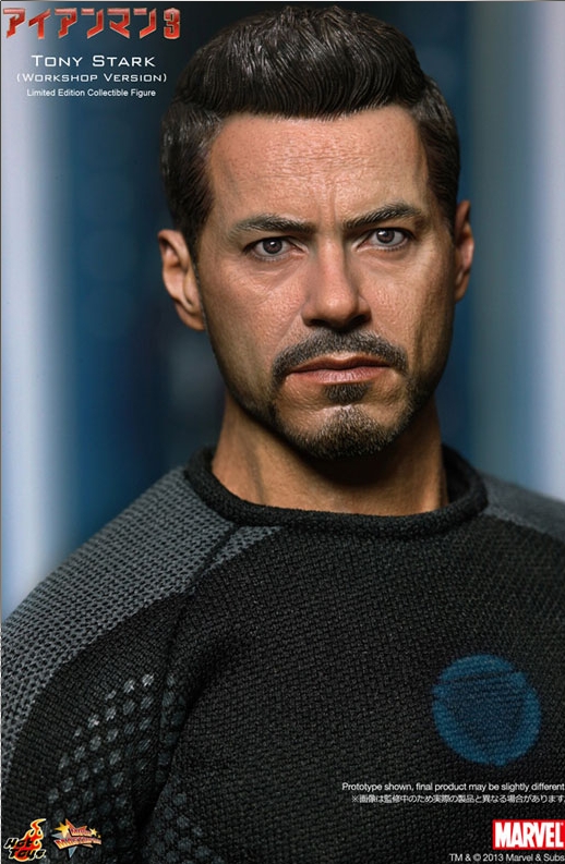
Realistic Avengers action figures
Read more: Realistic Avengers action figureshttp://kotaku.com/5911846/these-avengers-action-figures-look-so-real-youll-think-theyre-tiny-actors
http://www.sideshowtoy.com/?page_id=37555&ref=Avengers2012
http://www.sideshowtoy.com/?page_id=4489&sku=9017301&ref=ref=avengersLP_9017301#!prettyPhoto/0/
http://animagetoyznews.blogspot.co.nz/


COLOR
-
Björn Ottosson – OKHSV and OKHSL – Two new color spaces for color picking
Read more: Björn Ottosson – OKHSV and OKHSL – Two new color spaces for color pickinghttps://bottosson.github.io/misc/colorpicker
https://bottosson.github.io/posts/colorpicker/
https://www.smashingmagazine.com/2024/10/interview-bjorn-ottosson-creator-oklab-color-space/
One problem with sRGB is that in a gradient between blue and white, it becomes a bit purple in the middle of the transition. That’s because sRGB really isn’t created to mimic how the eye sees colors; rather, it is based on how CRT monitors work. That means it works with certain frequencies of red, green, and blue, and also the non-linear coding called gamma. It’s a miracle it works as well as it does, but it’s not connected to color perception. When using those tools, you sometimes get surprising results, like purple in the gradient.

There were also attempts to create simple models matching human perception based on XYZ, but as it turned out, it’s not possible to model all color vision that way. Perception of color is incredibly complex and depends, among other things, on whether it is dark or light in the room and the background color it is against. When you look at a photograph, it also depends on what you think the color of the light source is. The dress is a typical example of color vision being very context-dependent. It is almost impossible to model this perfectly.
I based Oklab on two other color spaces, CIECAM16 and IPT. I used the lightness and saturation prediction from CIECAM16, which is a color appearance model, as a target. I actually wanted to use the datasets used to create CIECAM16, but I couldn’t find them.
IPT was designed to have better hue uniformity. In experiments, they asked people to match light and dark colors, saturated and unsaturated colors, which resulted in a dataset for which colors, subjectively, have the same hue. IPT has a few other issues but is the basis for hue in Oklab.
In the Munsell color system, colors are described with three parameters, designed to match the perceived appearance of colors: Hue, Chroma and Value. The parameters are designed to be independent and each have a uniform scale. This results in a color solid with an irregular shape. The parameters are designed to be independent and each have a uniform scale. This results in a color solid with an irregular shape. Modern color spaces and models, such as CIELAB, Cam16 and Björn Ottosson own Oklab, are very similar in their construction.

By far the most used color spaces today for color picking are HSL and HSV, two representations introduced in the classic 1978 paper “Color Spaces for Computer Graphics”. HSL and HSV designed to roughly correlate with perceptual color properties while being very simple and cheap to compute.
Today HSL and HSV are most commonly used together with the sRGB color space.

One of the main advantages of HSL and HSV over the different Lab color spaces is that they map the sRGB gamut to a cylinder. This makes them easy to use since all parameters can be changed independently, without the risk of creating colors outside of the target gamut.

The main drawback on the other hand is that their properties don’t match human perception particularly well.
Reconciling these conflicting goals perfectly isn’t possible, but given that HSV and HSL don’t use anything derived from experiments relating to human perception, creating something that makes a better tradeoff does not seem unreasonable.
With this new lightness estimate, we are ready to look into the construction of Okhsv and Okhsl.


-
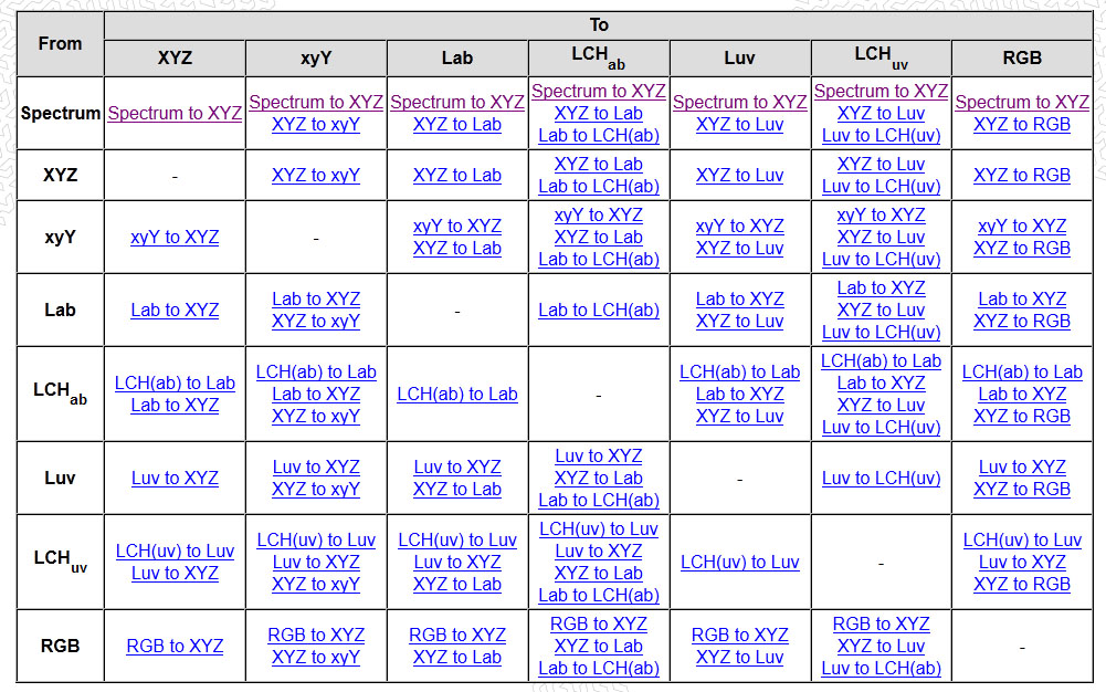
What is a Gamut or Color Space and why do I need to know about CIE
Read more: What is a Gamut or Color Space and why do I need to know about CIE

http://www.xdcam-user.com/2014/05/what-is-a-gamut-or-color-space-and-why-do-i-need-to-know-about-it/
In video terms gamut is normally related to as the full range of colours and brightness that can be either captured or displayed.
(more…)


LIGHTING
-
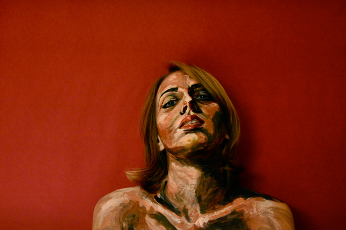
Composition – These are the basic lighting techniques you need to know for photography and film
Read more: Composition – These are the basic lighting techniques you need to know for photography and film
http://www.diyphotography.net/basic-lighting-techniques-need-know-photography-film/
Amongst the basic techniques, there’s…
1- Side lighting – Literally how it sounds, lighting a subject from the side when they’re faced toward you
2- Rembrandt lighting – Here the light is at around 45 degrees over from the front of the subject, raised and pointing down at 45 degrees
3- Back lighting – Again, how it sounds, lighting a subject from behind. This can help to add drama with silouettes
4- Rim lighting – This produces a light glowing outline around your subject
5- Key light – The main light source, and it’s not necessarily always the brightest light source
6- Fill light – This is used to fill in the shadows and provide detail that would otherwise be blackness
7- Cross lighting – Using two lights placed opposite from each other to light two subjects
-
Neural Microfacet Fields for Inverse Rendering
Read more: Neural Microfacet Fields for Inverse Renderinghttps://half-potato.gitlab.io/posts/nmf/

-
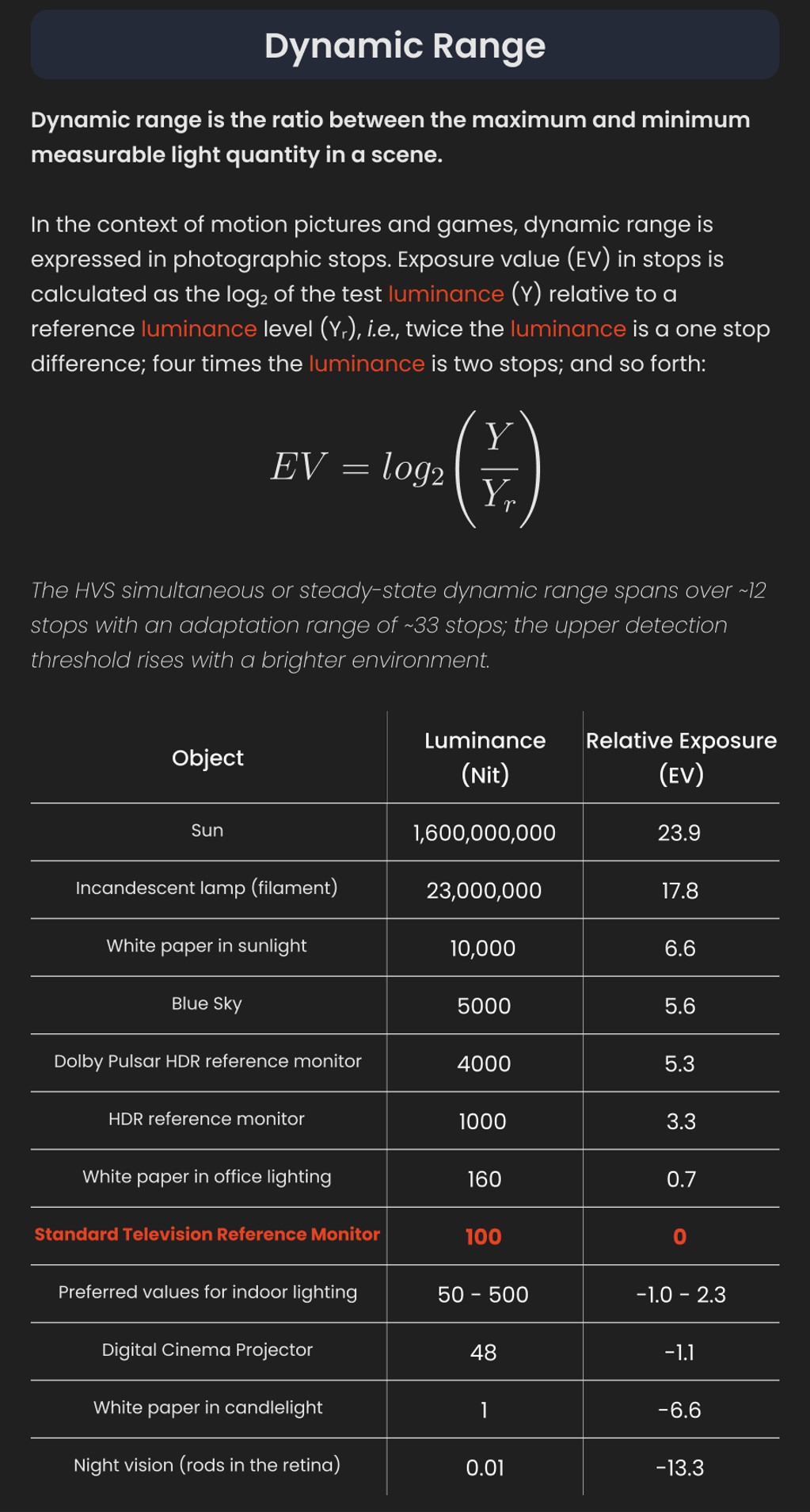
Convert between light exposure and intensity
Read more: Convert between light exposure and intensityimport math,sys def Exposure2Intensity(exposure): exp = float(exposure) result = math.pow(2,exp) print(result) Exposure2Intensity(0) def Intensity2Exposure(intensity): inarg = float(intensity) if inarg == 0: print("Exposure of zero intensity is undefined.") return if inarg < 1e-323: inarg = max(inarg, 1e-323) print("Exposure of negative intensities is undefined. Clamping to a very small value instead (1e-323)") result = math.log(inarg, 2) print(result) Intensity2Exposure(0.1)Why Exposure?
Exposure is a stop value that multiplies the intensity by 2 to the power of the stop. Increasing exposure by 1 results in double the amount of light.
Artists think in “stops.” Doubling or halving brightness is easy math and common in grading and look-dev.
Exposure counts doublings in whole stops:- +1 stop = ×2 brightness
- −1 stop = ×0.5 brightness
This gives perceptually even controls across both bright and dark values.
Why Intensity?
Intensity is linear.
It’s what render engines and compositors expect when:- Summing values
- Averaging pixels
- Multiplying or filtering pixel data
Use intensity when you need the actual math on pixel/light data.
Formulas (from your Python)
- Intensity from exposure: intensity = 2**exposure
- Exposure from intensity: exposure = log₂(intensity)
Guardrails:
- Intensity must be > 0 to compute exposure.
- If intensity = 0 → exposure is undefined.
- Clamp tiny values (e.g.
1e−323) before using log₂.
Use Exposure (stops) when…
- You want artist-friendly sliders (−5…+5 stops)
- Adjusting look-dev or grading in even stops
- Matching plates with quick ±1 stop tweaks
- Tweening brightness changes smoothly across ranges
Use Intensity (linear) when…
- Storing raw pixel/light values
- Multiplying textures or lights by a gain
- Performing sums, averages, and filters
- Feeding values to render engines expecting linear data
Examples
- +2 stops → 2**2 = 4.0 (×4)
- +1 stop → 2**1 = 2.0 (×2)
- 0 stop → 2**0 = 1.0 (×1)
- −1 stop → 2**(−1) = 0.5 (×0.5)
- −2 stops → 2**(−2) = 0.25 (×0.25)
- Intensity 0.1 → exposure = log₂(0.1) ≈ −3.32
Rule of thumb
Think in stops (exposure) for controls and matching.
Compute in linear (intensity) for rendering and math. -
Lighting Every Darkness with 3DGS: Fast Training and Real-Time Rendering and Denoising for HDR View Synthesis
Read more: Lighting Every Darkness with 3DGS: Fast Training and Real-Time Rendering and Denoising for HDR View Synthesishttps://srameo.github.io/projects/le3d/
LE3D is a method for real-time HDR view synthesis from RAW images. It is particularly effective for nighttime scenes.
https://github.com/Srameo/LE3D


COLLECTIONS
| Featured AI
| Design And Composition
| Explore posts
POPULAR SEARCHES
unreal | pipeline | virtual production | free | learn | photoshop | 360 | macro | google | nvidia | resolution | open source | hdri | real-time | photography basics | nuke
FEATURED POSTS
-
Daniele Tosti Interview for the magazine InCG, Taiwan, Issue 28, 201609
-
Jesse Zumstein – Jobs in games
-
Principles of Animation with Alan Becker, Dermot OConnor and Shaun Keenan
-
N8N.io – From Zero to Your First AI Agent in 25 Minutes
-
Free fonts
-
NVidia – High-Fidelity 3D Mesh Generation at Scale with Meshtron
-
Top 3D Printing Website Resources
-
AI and the Law – studiobinder.com – What is Fair Use: Definition, Policies, Examples and More
Social Links
DISCLAIMER – Links and images on this website may be protected by the respective owners’ copyright. All data submitted by users through this site shall be treated as freely available to share.
