


COMPOSITION
-
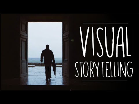
Composition and The Expressive Nature Of Light
Read more: Composition and The Expressive Nature Of Lighthttp://www.huffingtonpost.com/bill-danskin/post_12457_b_10777222.html
George Sand once said “ The artist vocation is to send light into the human heart.”

-
SlowMoVideo – How to make a slow motion shot with the open source program
Read more: SlowMoVideo – How to make a slow motion shot with the open source programhttp://slowmovideo.granjow.net/
slowmoVideo is an OpenSource program that creates slow-motion videos from your footage.
Slow motion cinematography is the result of playing back frames for a longer duration than they were exposed. For example, if you expose 240 frames of film in one second, then play them back at 24 fps, the resulting movie is 10 times longer (slower) than the original filmed event….
Film cameras are relatively simple mechanical devices that allow you to crank up the speed to whatever rate the shutter and pull-down mechanism allow. Some film cameras can operate at 2,500 fps or higher (although film shot in these cameras often needs some readjustment in postproduction). Video, on the other hand, is always captured, recorded, and played back at a fixed rate, with a current limit around 60fps. This makes extreme slow motion effects harder to achieve (and less elegant) on video, because slowing down the video results in each frame held still on the screen for a long time, whereas with high-frame-rate film there are plenty of frames to fill the longer durations of time. On video, the slow motion effect is more like a slide show than smooth, continuous motion.
One obvious solution is to shoot film at high speed, then transfer it to video (a case where film still has a clear advantage, sorry George). Another possibility is to cross dissolve or blur from one frame to the next. This adds a smooth transition from one still frame to the next. The blur reduces the sharpness of the image, and compared to slowing down images shot at a high frame rate, this is somewhat of a cheat. However, there isn’t much you can do about it until video can be recorded at much higher rates. Of course, many film cameras can’t shoot at high frame rates either, so the whole super-slow-motion endeavor is somewhat specialized no matter what medium you are using. (There are some high speed digital cameras available now that allow you to capture lots of digital frames directly to your computer, so technology is starting to catch up with film. However, this feature isn’t going to appear in consumer camcorders any time soon.)


DESIGN
-
Public Work – A search engine for free public domain content
Read more: Public Work – A search engine for free public domain contentExplore 100,000+ copyright-free images from The MET, New York Public Library, and other sources.


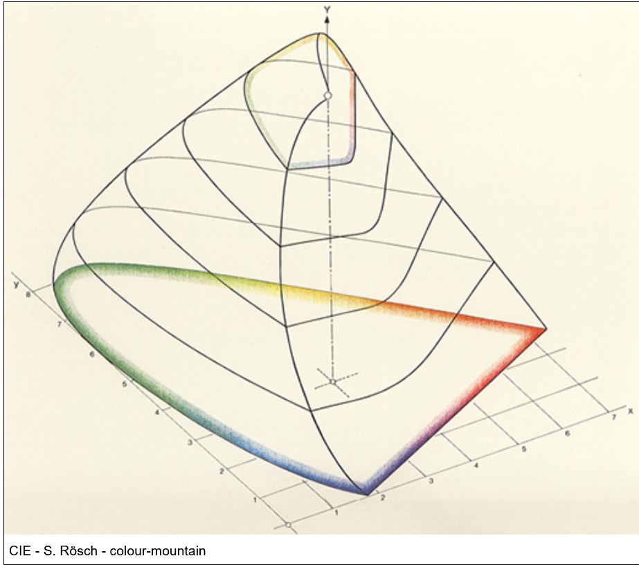
COLOR
-
Capturing textures albedo
Read more: Capturing textures albedoBuilding a Portable PBR Texture Scanner by Stephane Lb
http://rtgfx.com/pbr-texture-scanner/

How To Split Specular And Diffuse In Real Images, by John Hable
http://filmicworlds.com/blog/how-to-split-specular-and-diffuse-in-real-images/Capturing albedo using a Spectralon
https://www.activision.com/cdn/research/Real_World_Measurements_for_Call_of_Duty_Advanced_Warfare.pdfReal_World_Measurements_for_Call_of_Duty_Advanced_Warfare.pdf
Spectralon is a teflon-based pressed powderthat comes closest to being a pure Lambertian diffuse material that reflects 100% of all light. If we take an HDR photograph of the Spectralon alongside the material to be measured, we can derive thediffuse albedo of that material.

The process to capture diffuse reflectance is very similar to the one outlined by Hable.
1. We put a linear polarizing filter in front of the camera lens and a second linear polarizing filterin front of a modeling light or a flash such that the two filters are oriented perpendicular to eachother, i.e. cross polarized.
2. We place Spectralon close to and parallel with the material we are capturing and take brack-eted shots of the setup7. Typically, we’ll take nine photographs, from -4EV to +4EV in 1EVincrements.
3. We convert the bracketed shots to a linear HDR image. We found that many HDR packagesdo not produce an HDR image in which the pixel values are linear. PTGui is an example of apackage which does generate a linear HDR image. At this point, because of the cross polarization,the image is one of surface diffuse response.
4. We open the file in Photoshop and normalize the image by color picking the Spectralon, filling anew layer with that color and setting that layer to “Divide”. This sets the Spectralon to 1 in theimage. All other color values are relative to this so we can consider them as diffuse albedo.
-
StudioBinder.com – CRI color rendering index
Read more: StudioBinder.com – CRI color rendering indexwww.studiobinder.com/blog/what-is-color-rendering-index
“The Color Rendering Index is a measurement of how faithfully a light source reveals the colors of whatever it illuminates, it describes the ability of a light source to reveal the color of an object, as compared to the color a natural light source would provide. The highest possible CRI is 100. A CRI of 100 generally refers to a perfect black body, like a tungsten light source or the sun. ”


www.pixelsham.com/2021/04/28/types-of-film-lights-and-their-efficiency
-
What Is The Resolution and view coverage Of The human Eye. And what distance is TV at best?
Read more: What Is The Resolution and view coverage Of The human Eye. And what distance is TV at best?
https://www.discovery.com/science/mexapixels-in-human-eye
About 576 megapixels for the entire field of view.
Consider a view in front of you that is 90 degrees by 90 degrees, like looking through an open window at a scene. The number of pixels would be:
90 degrees * 60 arc-minutes/degree * 1/0.3 * 90 * 60 * 1/0.3 = 324,000,000 pixels (324 megapixels).At any one moment, you actually do not perceive that many pixels, but your eye moves around the scene to see all the detail you want. But the human eye really sees a larger field of view, close to 180 degrees. Let’s be conservative and use 120 degrees for the field of view. Then we would see:
120 * 120 * 60 * 60 / (0.3 * 0.3) = 576 megapixels.
Or.
7 megapixels for the 2 degree focus arc… + 1 megapixel for the rest.
https://clarkvision.com/articles/eye-resolution.html
Details in the post
-
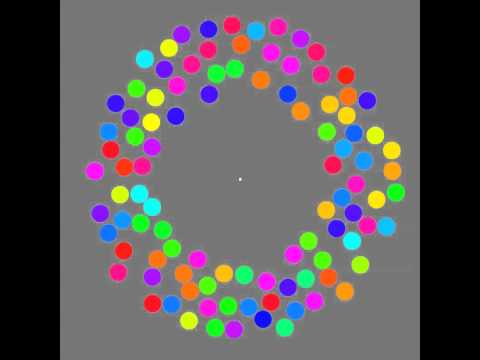
Mysterious animation wins best illusion of 2011 – Motion silencing illusion
Read more: Mysterious animation wins best illusion of 2011 – Motion silencing illusionThe 2011 Best Illusion of the Year uses motion to render color changes invisible, and so reveals a quirk in our visual systems that is new to scientists.
https://en.wikipedia.org/wiki/Motion_silencing_illusion
“It is a really beautiful effect, revealing something about how our visual system works that we didn’t know before,” said Daniel Simons, a professor at the University of Illinois, Champaign-Urbana. Simons studies visual cognition, and did not work on this illusion. Before its creation, scientists didn’t know that motion had this effect on perception, Simons said.
A viewer stares at a speck at the center of a ring of colored dots, which continuously change color. When the ring begins to rotate around the speck, the color changes appear to stop. But this is an illusion. For some reason, the motion causes our visual system to ignore the color changes. (You can, however, see the color changes if you follow the rotating circles with your eyes.)


LIGHTING
-
Disney’s Moana Island Scene – Free data set
Read more: Disney’s Moana Island Scene – Free data sethttps://www.disneyanimation.com/resources/moana-island-scene/
This data set contains everything necessary to render a version of the Motunui island featured in the 2016 film Moana.

-
IES Light Profiles and editing software
Read more: IES Light Profiles and editing softwarehttp://www.derekjenson.com/3d-blog/ies-light-profiles
https://ieslibrary.com/en/browse#ies
https://leomoon.com/store/shaders/ies-lights-pack
https://docs.arnoldrenderer.com/display/a5afmug/ai+photometric+light
IES profiles are useful for creating life-like lighting, as they can represent the physical distribution of light from any light source.
The IES format was created by the Illumination Engineering Society, and most lighting manufacturers provide IES profile for the lights they manufacture.


-
Bella – Fast Spectral Rendering
Read more: Bella – Fast Spectral Rendering
Bella works in spectral space, allowing effects such as BSDF wavelength dependency, diffraction, or atmosphere to be modeled far more accurately than in color space.

https://superrendersfarm.com/blog/uncategorized/bella-a-new-spectral-physically-based-renderer/
-
7 Easy Portrait Lighting Setups
Read more: 7 Easy Portrait Lighting Setups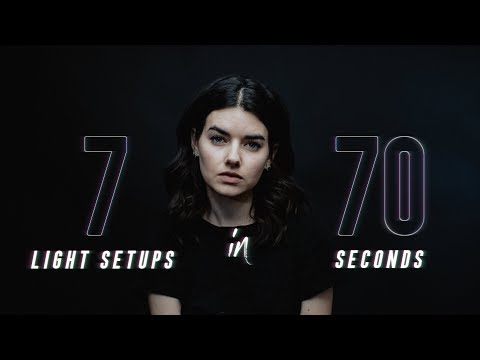
Butterfly
Loop
Rembrandt
Split
Rim
Broad
Short
-
Types of Film Lights and their efficiency – CRI, Color Temperature and Luminous Efficacy
Read more: Types of Film Lights and their efficiency – CRI, Color Temperature and Luminous Efficacynofilmschool.com/types-of-film-lights
“Not every light performs the same way. Lights and lighting are tricky to handle. You have to plan for every circumstance. But the good news is, lighting can be adjusted. Let’s look at different factors that affect lighting in every scene you shoot. “
Use CRI, Luminous Efficacy and color temperature controls to match your needs.
Color Temperature
Color temperature describes the “color” of white light by a light source radiated by a perfect black body at a given temperature measured in degrees Kelvinhttps://www.pixelsham.com/2019/10/18/color-temperature/
CRI
“The Color Rendering Index is a measurement of how faithfully a light source reveals the colors of whatever it illuminates, it describes the ability of a light source to reveal the color of an object, as compared to the color a natural light source would provide. The highest possible CRI is 100. A CRI of 100 generally refers to a perfect black body, like a tungsten light source or the sun. “https://www.studiobinder.com/blog/what-is-color-rendering-index
(more…) -
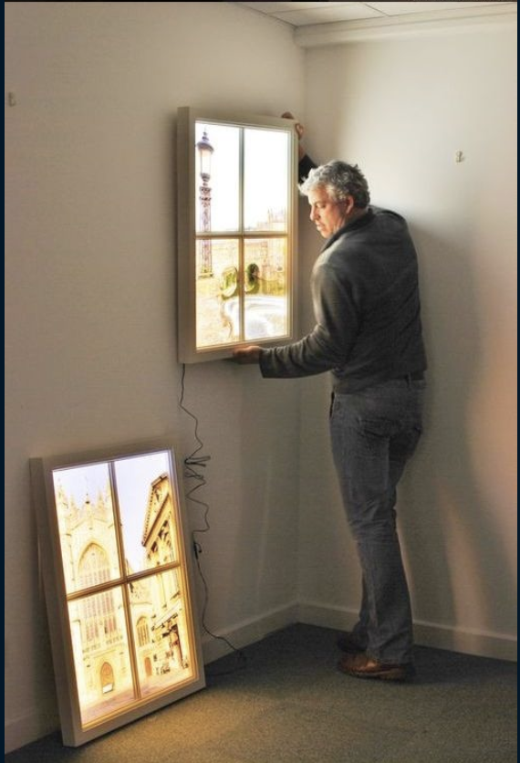
Polarised vs unpolarized filtering
Read more: Polarised vs unpolarized filteringA light wave that is vibrating in more than one plane is referred to as unpolarized light. …
Polarized light waves are light waves in which the vibrations occur in a single plane. The process of transforming unpolarized light into polarized light is known as polarization.

en.wikipedia.org/wiki/Polarizing_filter_(photography)
The most common use of polarized technology is to reduce lighting complexity on the subject.
(more…)
Details such as glare and hard edges are not removed, but greatly reduced.


COLLECTIONS
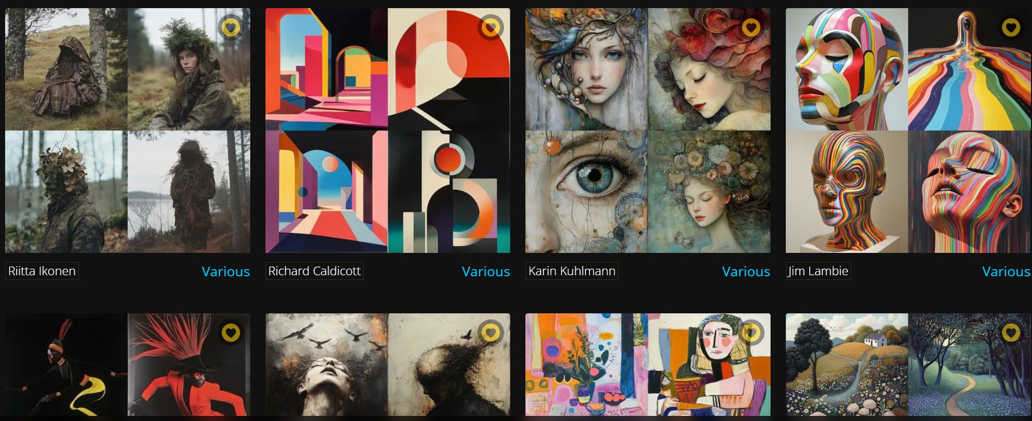
| Featured AI
| Design And Composition
| Explore posts
POPULAR SEARCHES
unreal | pipeline | virtual production | free | learn | photoshop | 360 | macro | google | nvidia | resolution | open source | hdri | real-time | photography basics | nuke
FEATURED POSTS
-
Eyeline Labs VChain – Chain-of-Visual-Thought for Reasoning in Video Generation for better AI physics
-
Animation/VFX/Game Industry JOB POSTINGS by Chris Mayne
-
The Public Domain Is Working Again — No Thanks To Disney
-
Top 3D Printing Website Resources
-
VFX pipeline – Render Wall Farm management topics
-
N8N.io – From Zero to Your First AI Agent in 25 Minutes
-
UV maps
-
How do LLMs like ChatGPT (Generative Pre-Trained Transformer) work? Explained by Deep-Fake Ryan Gosling
Social Links
DISCLAIMER – Links and images on this website may be protected by the respective owners’ copyright. All data submitted by users through this site shall be treated as freely available to share.
