


COMPOSITION
-
StudioBinder – Roger Deakins on How to Choose a Camera Lens — Cinematography Composition Techniques
Read more: StudioBinder – Roger Deakins on How to Choose a Camera Lens — Cinematography Composition Techniques
https://www.studiobinder.com/blog/camera-lens-buying-guide/
https://www.studiobinder.com/blog/e-books/camera-lenses-explained-volume-1-ebook


DESIGN


COLOR
-
Rec-2020 – TVs new color gamut standard used by Dolby Vision?
Read more: Rec-2020 – TVs new color gamut standard used by Dolby Vision?https://www.hdrsoft.com/resources/dri.html#bit-depth

The dynamic range is a ratio between the maximum and minimum values of a physical measurement. Its definition depends on what the dynamic range refers to.
For a scene: Dynamic range is the ratio between the brightest and darkest parts of the scene.
For a camera: Dynamic range is the ratio of saturation to noise. More specifically, the ratio of the intensity that just saturates the camera to the intensity that just lifts the camera response one standard deviation above camera noise.
For a display: Dynamic range is the ratio between the maximum and minimum intensities emitted from the screen.
The Dynamic Range of real-world scenes can be quite high — ratios of 100,000:1 are common in the natural world. An HDR (High Dynamic Range) image stores pixel values that span the whole tonal range of real-world scenes. Therefore, an HDR image is encoded in a format that allows the largest range of values, e.g. floating-point values stored with 32 bits per color channel. Another characteristics of an HDR image is that it stores linear values. This means that the value of a pixel from an HDR image is proportional to the amount of light measured by the camera.
For TVs HDR is great, but it’s not the only new TV feature worth discussing.
(more…) -
The Color of Infinite Temperature
Read more: The Color of Infinite TemperatureThis is the color of something infinitely hot.

Of course you’d instantly be fried by gamma rays of arbitrarily high frequency, but this would be its spectrum in the visible range.
johncarlosbaez.wordpress.com/2022/01/16/the-color-of-infinite-temperature/
This is also the color of a typical neutron star. They’re so hot they look the same.
It’s also the color of the early Universe!This was worked out by David Madore.

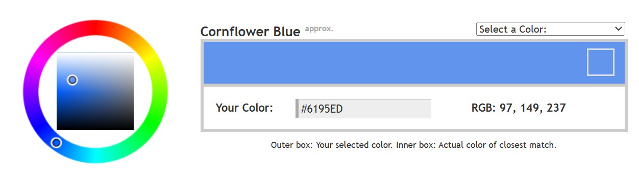
The color he got is sRGB(148,177,255).
www.htmlcsscolor.com/hex/94B1FFAnd according to the experts who sip latte all day and make up names for colors, this color is called ‘Perano’.
-
Tim Kang – calibrated white light values in sRGB color space
Read more: Tim Kang – calibrated white light values in sRGB color space8bit sRGB encoded
2000K 255 139 22
2700K 255 172 89
3000K 255 184 109
3200K 255 190 122
4000K 255 211 165
4300K 255 219 178
D50 255 235 205
D55 255 243 224
D5600 255 244 227
D6000 255 249 240
D65 255 255 255
D10000 202 221 255
D20000 166 196 2558bit Rec709 Gamma 2.4
2000K 255 145 34
2700K 255 177 97
3000K 255 187 117
3200K 255 193 129
4000K 255 214 170
4300K 255 221 182
D50 255 236 208
D55 255 243 226
D5600 255 245 229
D6000 255 250 241
D65 255 255 255
D10000 204 222 255
D20000 170 199 2558bit Display P3 encoded
2000K 255 154 63
2700K 255 185 109
3000K 255 195 127
3200K 255 201 138
4000K 255 219 176
4300K 255 225 187
D50 255 239 212
D55 255 245 228
D5600 255 246 231
D6000 255 251 242
D65 255 255 255
D10000 208 223 255
D20000 175 199 25510bit Rec2020 PQ (100 nits)
2000K 520 435 273
2700K 520 466 358
3000K 520 475 384
3200K 520 480 399
4000K 520 495 446
4300K 520 500 458
D50 520 510 482
D55 520 514 497
D5600 520 514 500
D6000 520 517 509
D65 520 520 520
D10000 479 489 520
D20000 448 464 520


![[gamma correction test]](http://www.madore.org/~david/misc/color/gammatest.png "sRGB gamma correction test")


LIGHTING
-
3D Lighting Tutorial by Amaan Kram
Read more: 3D Lighting Tutorial by Amaan Kramhttp://www.amaanakram.com/lightingT/part1.htm
The goals of lighting in 3D computer graphics are more or less the same as those of real world lighting.
Lighting serves a basic function of bringing out, or pushing back the shapes of objects visible from the camera’s view.
It gives a two-dimensional image on the monitor an illusion of the third dimension-depth.But it does not just stop there. It gives an image its personality, its character. A scene lit in different ways can give a feeling of happiness, of sorrow, of fear etc., and it can do so in dramatic or subtle ways. Along with personality and character, lighting fills a scene with emotion that is directly transmitted to the viewer.
Trying to simulate a real environment in an artificial one can be a daunting task. But even if you make your 3D rendering look absolutely photo-realistic, it doesn’t guarantee that the image carries enough emotion to elicit a “wow” from the people viewing it.
Making 3D renderings photo-realistic can be hard. Putting deep emotions in them can be even harder. However, if you plan out your lighting strategy for the mood and emotion that you want your rendering to express, you make the process easier for yourself.
Each light source can be broken down in to 4 distinct components and analyzed accordingly.
· Intensity
· Direction
· Color
· SizeThe overall thrust of this writing is to produce photo-realistic images by applying good lighting techniques.

-
Simulon – a Hollywood production studio app in the hands of an independent creator with access to consumer hardware, LDRi to HDRi through ML
Read more: Simulon – a Hollywood production studio app in the hands of an independent creator with access to consumer hardware, LDRi to HDRi through MLDivesh Naidoo: The video below was made with a live in-camera preview and auto-exposure matching, no camera solve, no HDRI capture and no manual compositing setup. Using the new Simulon phone app.
LDR to HDR through ML
https://simulon.typeform.com/betatest
(more…)Process example


COLLECTIONS
| Featured AI
| Design And Composition
| Explore posts
POPULAR SEARCHES
unreal | pipeline | virtual production | free | learn | photoshop | 360 | macro | google | nvidia | resolution | open source | hdri | real-time | photography basics | nuke
FEATURED POSTS
-
Convert 2D Images or Text to 3D Models
-
White Balance is Broken!
-
Photography basics: Exposure Value vs Photographic Exposure vs Il/Luminance vs Pixel luminance measurements
-
Methods for creating motion blur in Stop motion
-
AI and the Law – Netflix : Using Generative AI in Content Production
-
AnimationXpress.com interviews Daniele Tosti for TheCgCareer.com channel
-
Black Body color aka the Planckian Locus curve for white point eye perception
-
Glossary of Lighting Terms – cheat sheet
Social Links
DISCLAIMER – Links and images on this website may be protected by the respective owners’ copyright. All data submitted by users through this site shall be treated as freely available to share.
