COMPOSITION
-
SlowMoVideo – How to make a slow motion shot with the open source program
http://slowmovideo.granjow.net/
slowmoVideo is an OpenSource program that creates slow-motion videos from your footage.
Slow motion cinematography is the result of playing back frames for a longer duration than they were exposed. For example, if you expose 240 frames of film in one second, then play them back at 24 fps, the resulting movie is 10 times longer (slower) than the original filmed event….
Film cameras are relatively simple mechanical devices that allow you to crank up the speed to whatever rate the shutter and pull-down mechanism allow. Some film cameras can operate at 2,500 fps or higher (although film shot in these cameras often needs some readjustment in postproduction). Video, on the other hand, is always captured, recorded, and played back at a fixed rate, with a current limit around 60fps. This makes extreme slow motion effects harder to achieve (and less elegant) on video, because slowing down the video results in each frame held still on the screen for a long time, whereas with high-frame-rate film there are plenty of frames to fill the longer durations of time. On video, the slow motion effect is more like a slide show than smooth, continuous motion.
One obvious solution is to shoot film at high speed, then transfer it to video (a case where film still has a clear advantage, sorry George). Another possibility is to cross dissolve or blur from one frame to the next. This adds a smooth transition from one still frame to the next. The blur reduces the sharpness of the image, and compared to slowing down images shot at a high frame rate, this is somewhat of a cheat. However, there isn’t much you can do about it until video can be recorded at much higher rates. Of course, many film cameras can’t shoot at high frame rates either, so the whole super-slow-motion endeavor is somewhat specialized no matter what medium you are using. (There are some high speed digital cameras available now that allow you to capture lots of digital frames directly to your computer, so technology is starting to catch up with film. However, this feature isn’t going to appear in consumer camcorders any time soon.)
DESIGN
COLOR
-
Photography basics: Lumens vs Candelas (candle) vs Lux vs FootCandle vs Watts vs Irradiance vs Illuminance
Read more: Photography basics: Lumens vs Candelas (candle) vs Lux vs FootCandle vs Watts vs Irradiance vs Illuminancehttps://www.translatorscafe.com/unit-converter/en-US/illumination/1-11/
The power output of a light source is measured using the unit of watts W. This is a direct measure to calculate how much power the light is going to drain from your socket and it is not relatable to the light brightness itself.
The amount of energy emitted from it per second. That energy comes out in a form of photons which we can crudely represent with rays of light coming out of the source. The higher the power the more rays emitted from the source in a unit of time.
Not all energy emitted is visible to the human eye, so we often rely on photometric measurements, which takes in account the sensitivity of human eye to different wavelenghts
Details in the post
(more…) -
THOMAS MANSENCAL – The Apparent Simplicity of RGB Rendering
https://thomasmansencal.substack.com/p/the-apparent-simplicity-of-rgb-rendering
The primary goal of physically-based rendering (PBR) is to create a simulation that accurately reproduces the imaging process of electro-magnetic spectrum radiation incident to an observer. This simulation should be indistinguishable from reality for a similar observer.
Because a camera is not sensitive to incident light the same way than a human observer, the images it captures are transformed to be colorimetric. A project might require infrared imaging simulation, a portion of the electro-magnetic spectrum that is invisible to us. Radically different observers might image the same scene but the act of observing does not change the intrinsic properties of the objects being imaged. Consequently, the physical modelling of the virtual scene should be independent of the observer.
-
About color: What is a LUT
Read more: About color: What is a LUThttp://www.lightillusion.com/luts.html
https://www.shutterstock.com/blog/how-use-luts-color-grading
A LUT (Lookup Table) is essentially the modifier between two images, the original image and the displayed image, based on a mathematical formula. Basically conversion matrices of different complexities. There are different types of LUTS – viewing, transform, calibration, 1D and 3D.
-
Weta Digital – Manuka Raytracer and Gazebo GPU renderers – pipeline
Read more: Weta Digital – Manuka Raytracer and Gazebo GPU renderers – pipelinehttps://jo.dreggn.org/home/2018_manuka.pdf
http://www.fxguide.com/featured/manuka-weta-digitals-new-renderer/
The Manuka rendering architecture has been designed in the spirit of the classic reyes rendering architecture. In its core, reyes is based on stochastic rasterisation of micropolygons, facilitating depth of field, motion blur, high geometric complexity,and programmable shading.
This is commonly achieved with Monte Carlo path tracing, using a paradigm often called shade-on-hit, in which the renderer alternates tracing rays with running shaders on the various ray hits. The shaders take the role of generating the inputs of the local material structure which is then used bypath sampling logic to evaluate contributions and to inform what further rays to cast through the scene.
Over the years, however, the expectations have risen substantially when it comes to image quality. Computing pictures which are indistinguishable from real footage requires accurate simulation of light transport, which is most often performed using some variant of Monte Carlo path tracing. Unfortunately this paradigm requires random memory accesses to the whole scene and does not lend itself well to a rasterisation approach at all.
Manuka is both a uni-directional and bidirectional path tracer and encompasses multiple importance sampling (MIS). Interestingly, and importantly for production character skin work, it is the first major production renderer to incorporate spectral MIS in the form of a new ‘Hero Spectral Sampling’ technique, which was recently published at Eurographics Symposium on Rendering 2014.
Manuka propose a shade-before-hit paradigm in-stead and minimise I/O strain (and some memory costs) on the system, leveraging locality of reference by running pattern generation shaders before we execute light transport simulation by path sampling, “compressing” any bvh structure as needed, and as such also limiting duplication of source data.
The difference with reyes is that instead of baking colors into the geometry like in Reyes, manuka bakes surface closures. This means that light transport is still calculated with path tracing, but all texture lookups etc. are done up-front and baked into the geometry.The main drawback with this method is that geometry has to be tessellated to its highest, stable topology before shading can be evaluated properly. As such, the high cost to first pixel. Even a basic 4 vertices square becomes a much more complex model with this approach.
Manuka use the RenderMan Shading Language (rsl) for programmable shading [Pixar Animation Studios 2015], but we do not invoke rsl shaders when intersecting a ray with a surface (often called shade-on-hit). Instead, we pre-tessellate and pre-shade all the input geometry in the front end of the renderer.
This way, we can efficiently order shading computations to sup-port near-optimal texture locality, vectorisation, and parallelism. This system avoids repeated evaluation of shaders at the same surface point, and presents a minimal amount of memory to be accessed during light transport time. An added benefit is that the acceleration structure for ray tracing (abounding volume hierarchy, bvh) is built once on the final tessellated geometry, which allows us to ray trace more efficiently than multi-level bvhs and avoids costly caching of on-demand tessellated micropolygons and the associated scheduling issues.For the shading reasons above, in terms of AOVs, the studio approach is to succeed at combining complex shading with ray paths in the render rather than pass a multi-pass render to compositing.
For the Spectral Rendering component. The light transport stage is fully spectral, using a continuously sampled wavelength which is traced with each path and used to apply the spectral camera sensitivity of the sensor. This allows for faithfully support any degree of observer metamerism as the camera footage they are intended to match as well as complex materials which require wavelength dependent phenomena such as diffraction, dispersion, interference, iridescence, or chromatic extinction and Rayleigh scattering in participating media.
As opposed to the original reyes paper, we use bilinear interpolation of these bsdf inputs later when evaluating bsdfs per pathv ertex during light transport4. This improves temporal stability of geometry which moves very slowly with respect to the pixel raster
In terms of the pipeline, everything rendered at Weta was already completely interwoven with their deep data pipeline. Manuka very much was written with deep data in mind. Here, Manuka not so much extends the deep capabilities, rather it fully matches the already extremely complex and powerful setup Weta Digital already enjoy with RenderMan. For example, an ape in a scene can be selected, its ID is available and a NUKE artist can then paint in 3D say a hand and part of the way up the neutral posed ape.
We called our system Manuka, as a respectful nod to reyes: we had heard a story froma former ILM employee about how reyes got its name from how fond the early Pixar people were of their lunches at Point Reyes, and decided to name our system after our surrounding natural environment, too. Manuka is a kind of tea tree very common in New Zealand which has very many very small leaves, in analogy to micropolygons ina tree structure for ray tracing. It also happens to be the case that Weta Digital’s main site is on Manuka Street.
-
Colour – MacBeth Chart Checker Detection
Read more: Colour – MacBeth Chart Checker Detectiongithub.com/colour-science/colour-checker-detection
A Python package implementing various colour checker detection algorithms and related utilities.
-
Photography basics: Why Use a (MacBeth) Color Chart?
Read more: Photography basics: Why Use a (MacBeth) Color Chart?Start here: https://www.pixelsham.com/2013/05/09/gretagmacbeth-color-checker-numeric-values/
https://www.studiobinder.com/blog/what-is-a-color-checker-tool/
In LightRoom
in Final Cut
in Nuke
Note: In Foundry’s Nuke, the software will map 18% gray to whatever your center f/stop is set to in the viewer settings (f/8 by default… change that to EV by following the instructions below).
You can experiment with this by attaching an Exposure node to a Constant set to 0.18, setting your viewer read-out to Spotmeter, and adjusting the stops in the node up and down. You will see that a full stop up or down will give you the respective next value on the aperture scale (f8, f11, f16 etc.).One stop doubles or halves the amount or light that hits the filmback/ccd, so everything works in powers of 2.
So starting with 0.18 in your constant, you will see that raising it by a stop will give you .36 as a floating point number (in linear space), while your f/stop will be f/11 and so on.If you set your center stop to 0 (see below) you will get a relative readout in EVs, where EV 0 again equals 18% constant gray.
In other words. Setting the center f-stop to 0 means that in a neutral plate, the middle gray in the macbeth chart will equal to exposure value 0. EV 0 corresponds to an exposure time of 1 sec and an aperture of f/1.0.
This will set the sun usually around EV12-17 and the sky EV1-4 , depending on cloud coverage.
To switch Foundry’s Nuke’s SpotMeter to return the EV of an image, click on the main viewport, and then press s, this opens the viewer’s properties. Now set the center f-stop to 0 in there. And the SpotMeter in the viewport will change from aperture and fstops to EV.
LIGHTING
-
Photography basics: Color Temperature and White Balance
Read more: Photography basics: Color Temperature and White BalanceColor Temperature of a light source describes the spectrum of light which is radiated from a theoretical “blackbody” (an ideal physical body that absorbs all radiation and incident light – neither reflecting it nor allowing it to pass through) with a given surface temperature.
https://en.wikipedia.org/wiki/Color_temperature
Or. Most simply it is a method of describing the color characteristics of light through a numerical value that corresponds to the color emitted by a light source, measured in degrees of Kelvin (K) on a scale from 1,000 to 10,000.
More accurately. The color temperature of a light source is the temperature of an ideal backbody that radiates light of comparable hue to that of the light source.
As such, the color temperature of a light source is a numerical measurement of its color appearance. It is based on the principle that any object will emit light if it is heated to a high enough temperature, and that the color of that light will shift in a predictable manner as the temperature is increased. The system is based on the color changes of a theoretical “blackbody radiator” as it is heated from a cold black to a white hot state.
So, why do we measure the hue of the light as a “temperature”? This was started in the late 1800s, when the British physicist William Kelvin heated a block of carbon. It glowed in the heat, producing a range of different colors at different temperatures. The black cube first produced a dim red light, increasing to a brighter yellow as the temperature went up, and eventually produced a bright blue-white glow at the highest temperatures. In his honor, Color Temperatures are measured in degrees Kelvin, which are a variation on Centigrade degrees. Instead of starting at the temperature water freezes, the Kelvin scale starts at “absolute zero,” which is -273 Centigrade.
More about black bodies here: https://www.pixelsham.com/2013/03/14/black-body-color
Details in the post
-
Outpost VFX lighting tips
Read more: Outpost VFX lighting tipswww.outpost-vfx.com/en/news/18-pro-tips-and-tricks-for-lighting
Get as much information regarding your plate lighting as possible
- Always use a reference
- Replicate what is happening in real life
- Invest into a solid HDRI
- Start Simple
- Observe real world lighting, photography and cinematography
- Don’t neglect the theory
- Learn the difference between realism and photo-realism.
- Keep your scenes organised
-
What is the Light Field?
Read more: What is the Light Field?http://lightfield-forum.com/what-is-the-lightfield/
The light field consists of the total of all light rays in 3D space, flowing through every point and in every direction.
How to Record a Light Field
- a single, robotically controlled camera
- a rotating arc of cameras
- an array of cameras or camera modules
- a single camera or camera lens fitted with a microlens array
-
HDRI Median Cut plugin
www.hdrlabs.com/picturenaut/plugins.html
Note. The Median Cut algorithm is typically used for color quantization, which involves reducing the number of colors in an image while preserving its visual quality. It doesn’t directly provide a way to identify the brightest areas in an image. However, if you’re interested in identifying the brightest areas, you might want to look into other methods like thresholding, histogram analysis, or edge detection, through openCV for example.
Here is an openCV example:
# bottom left coordinates = 0,0 import numpy as np import cv2 # Load the HDR or EXR image image = cv2.imread('your_image_path.exr', cv2.IMREAD_UNCHANGED) # Load as-is without modification # Calculate the luminance from the HDR channels (assuming RGB format) luminance = np.dot(image[..., :3], [0.299, 0.587, 0.114]) # Set a threshold value based on estimated EV threshold_value = 2.4 # Estimated threshold value based on 4.8 EV # Apply the threshold to identify bright areas # The
luminance
array contains the calculated luminance values for each pixel in the image. # Thethreshold_value
is a user-defined value that represents a cutoff point, separating "bright" and "dark" areas in terms of perceived luminance.thresholded = (luminance > threshold_value) * 255 # Convert the thresholded image to uint8 for contour detection thresholded = thresholded.astype(np.uint8) # Find contours of the bright areas contours, _ = cv2.findContours(thresholded, cv2.RETR_EXTERNAL, cv2.CHAIN_APPROX_SIMPLE) # Create a list to store the bounding boxes of bright areas bright_areas = [] # Iterate through contours and extract bounding boxes for contour in contours: x, y, w, h = cv2.boundingRect(contour) # Adjust y-coordinate based on bottom-left origin y_bottom_left_origin = image.shape[0] - (y + h) bright_areas.append((x, y_bottom_left_origin, x + w, y_bottom_left_origin + h)) # Store as (x1, y1, x2, y2) # Print the identified bright areas print("Bright Areas (x1, y1, x2, y2):") for area in bright_areas: print(area)
More details
Luminance and Exposure in an EXR Image:
- An EXR (Extended Dynamic Range) image format is often used to store high dynamic range (HDR) images that contain a wide range of luminance values, capturing both dark and bright areas.
- Luminance refers to the perceived brightness of a pixel in an image. In an RGB image, luminance is often calculated using a weighted sum of the red, green, and blue channels, where different weights are assigned to each channel to account for human perception.
- In an EXR image, the pixel values can represent radiometrically accurate scene values, including actual radiance or irradiance levels. These values are directly related to the amount of light emitted or reflected by objects in the scene.
The luminance line is calculating the luminance of each pixel in the image using a weighted sum of the red, green, and blue channels. The three float values [0.299, 0.587, 0.114] are the weights used to perform this calculation.
These weights are based on the concept of luminosity, which aims to approximate the perceived brightness of a color by taking into account the human eye’s sensitivity to different colors. The values are often derived from the NTSC (National Television System Committee) standard, which is used in various color image processing operations.
Here’s the breakdown of the float values:
- 0.299: Weight for the red channel.
- 0.587: Weight for the green channel.
- 0.114: Weight for the blue channel.
The weighted sum of these channels helps create a grayscale image where the pixel values represent the perceived brightness. This technique is often used when converting a color image to grayscale or when calculating luminance for certain operations, as it takes into account the human eye’s sensitivity to different colors.
For the threshold, remember that the exact relationship between EV values and pixel values can depend on the tone-mapping or normalization applied to the HDR image, as well as the dynamic range of the image itself.
To establish a relationship between exposure and the threshold value, you can consider the relationship between linear and logarithmic scales:
- Linear and Logarithmic Scales:
- Exposure values in an EXR image are often represented in logarithmic scales, such as EV (exposure value). Each increment in EV represents a doubling or halving of the amount of light captured.
- Threshold values for luminance thresholding are usually linear, representing an actual luminance level.
- Conversion Between Scales:
- To establish a mathematical relationship, you need to convert between the logarithmic exposure scale and the linear threshold scale.
- One common method is to use a power function. For instance, you can use a power function to convert EV to a linear intensity value.
threshold_value = base_value * (2 ** EV)
Here,
EV
is the exposure value,base_value
is a scaling factor that determines the relationship between EV and threshold_value, and2 ** EV
is used to convert the logarithmic EV to a linear intensity value. - Choosing the Base Value:
- The
base_value
factor should be determined based on the dynamic range of your EXR image and the specific luminance values you are dealing with. - You may need to experiment with different values of
base_value
to achieve the desired separation of bright areas from the rest of the image.
- The
Let’s say you have an EXR image with a dynamic range of 12 EV, which is a common range for many high dynamic range images. In this case, you want to set a threshold value that corresponds to a certain number of EV above the middle gray level (which is often considered to be around 0.18).
Here’s an example of how you might determine a
base_value
to achieve this:# Define the dynamic range of the image in EV dynamic_range = 12 # Choose the desired number of EV above middle gray for thresholding desired_ev_above_middle_gray = 2 # Calculate the threshold value based on the desired EV above middle gray threshold_value = 0.18 * (2 ** (desired_ev_above_middle_gray / dynamic_range)) print("Threshold Value:", threshold_value)
COLLECTIONS
| Featured AI
| Design And Composition
| Explore posts
POPULAR SEARCHES
unreal | pipeline | virtual production | free | learn | photoshop | 360 | macro | google | nvidia | resolution | open source | hdri | real-time | photography basics | nuke
FEATURED POSTS
-
Scene Referred vs Display Referred color workflows
-
PixelSham – Introduction to Python 2022
-
Cinematographers Blueprint 300dpi poster
-
Methods for creating motion blur in Stop motion
-
GretagMacbeth Color Checker Numeric Values and Middle Gray
-
Daniele Tosti Interview for the magazine InCG, Taiwan, Issue 28, 201609
-
Eddie Yoon – There’s a big misconception about AI creative
-
Top 3D Printing Website Resources
Social Links
DISCLAIMER – Links and images on this website may be protected by the respective owners’ copyright. All data submitted by users through this site shall be treated as freely available to share.
