


COMPOSITION


DESIGN
-
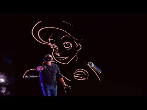
Glenn Marshall – The Crow
Read more: Glenn Marshall – The Crow
Created with AI ‘Style Transfer’ processes to transform video footage into AI video art.
-
Arminas Valunas – “Coca-Cola: Wherever you are.”
Read more: Arminas Valunas – “Coca-Cola: Wherever you are.”Arminas created this using Juggernaut Xl model and QR Code Monster SDXL ControlNet.
His pipeline:
Static Images – Forge UI.
Upscaled with Leonardo AI universal upscaler.
Animated with Runway ML and Minimax.
Video upscale – Topaz Video AI.
Composited in Adobe Premiere.
Juggernaut Xl download here:
https://civitai.com/models/133005/juggernaut-xl
QR Code Monster SDXL:
https://civitai.com/models/197247?modelVersionId=221829


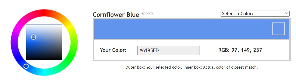
COLOR
-
PTGui 13 beta adds control through a Patch Editor
Read more: PTGui 13 beta adds control through a Patch EditorAdditions:
- Patch Editor (PTGui Pro)
- DNG output
- Improved RAW / DNG handling
- JPEG 2000 support
- Performance improvements

-
Paul Debevec, Chloe LeGendre, Lukas Lepicovsky – Jointly Optimizing Color Rendition and In-Camera Backgrounds in an RGB Virtual Production Stage
Read more: Paul Debevec, Chloe LeGendre, Lukas Lepicovsky – Jointly Optimizing Color Rendition and In-Camera Backgrounds in an RGB Virtual Production Stagehttps://arxiv.org/pdf/2205.12403.pdf
RGB LEDs vs RGBWP (RGB + lime + phospor converted amber) LEDs
Local copy:
-
Christopher Butler – Understanding the Eye-Mind Connection – Vision is a mental process
Read more: Christopher Butler – Understanding the Eye-Mind Connection – Vision is a mental processhttps://www.chrbutler.com/understanding-the-eye-mind-connection
The intricate relationship between the eyes and the brain, often termed the eye-mind connection, reveals that vision is predominantly a cognitive process. This understanding has profound implications for fields such as design, where capturing and maintaining attention is paramount. This essay delves into the nuances of visual perception, the brain’s role in interpreting visual data, and how this knowledge can be applied to effective design strategies.
This cognitive aspect of vision is evident in phenomena such as optical illusions, where the brain interprets visual information in a way that contradicts physical reality. These illusions underscore that what we “see” is not merely a direct recording of the external world but a constructed experience shaped by cognitive processes.
Understanding the cognitive nature of vision is crucial for effective design. Designers must consider how the brain processes visual information to create compelling and engaging visuals. This involves several key principles:
- Attention and Engagement
- Visual Hierarchy
- Cognitive Load Management
- Context and Meaning


LIGHTING
-
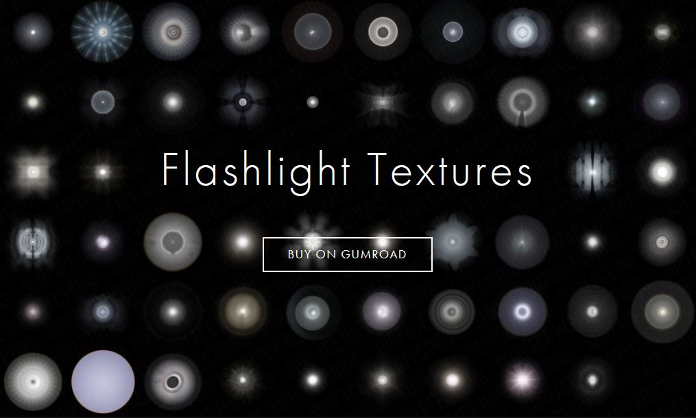
Custom bokeh in a raytraced DOF render
Read more: Custom bokeh in a raytraced DOF render

To achieve a custom pinhole camera effect with a custom bokeh in Arnold Raytracer, you can follow these steps:
- Set the render camera with a focal length around 50 (or as needed)
- Set the F-Stop to a high value (e.g., 22).
- Set the focus distance as you require
- Turn on DOF
- Place a plane a few cm in front of the camera.
- Texture the plane with a transparent shape at the center of it. (Transmission with no specular roughness)
-
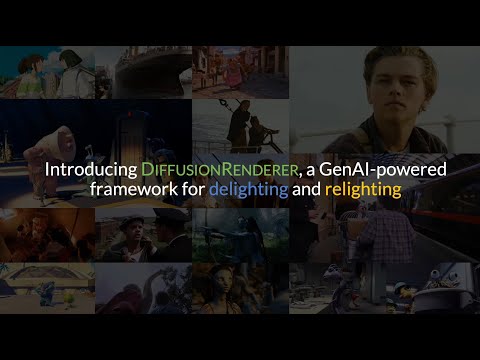
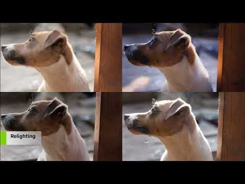
NVidia DiffusionRenderer – Neural Inverse and Forward Rendering with Video Diffusion Models. How NVIDIA reimagined relighting
Read more: NVidia DiffusionRenderer – Neural Inverse and Forward Rendering with Video Diffusion Models. How NVIDIA reimagined relightinghttps://www.fxguide.com/quicktakes/diffusing-reality-how-nvidia-reimagined-relighting/
https://research.nvidia.com/labs/toronto-ai/DiffusionRenderer/
-
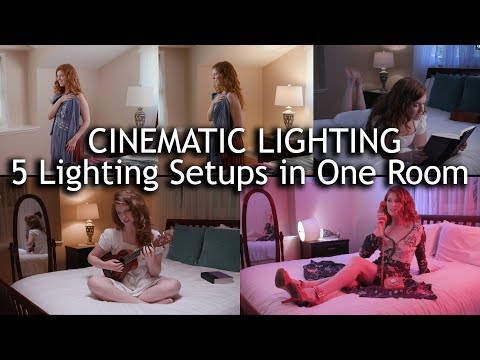
9 Best Hacks to Make a Cinematic Video with Any Camera
Read more: 9 Best Hacks to Make a Cinematic Video with Any Camerahttps://www.flexclip.com/learn/cinematic-video.html
- Frame Your Shots to Create Depth
- Create Shallow Depth of Field
- Avoid Shaky Footage and Use Flexible Camera Movements
- Properly Use Slow Motion
- Use Cinematic Lighting Techniques
- Apply Color Grading
- Use Cinematic Music and SFX
- Add Cinematic Fonts and Text Effects
- Create the Cinematic Bar at the Top and the Bottom


COLLECTIONS
| Featured AI
| Design And Composition
| Explore posts
POPULAR SEARCHES
unreal | pipeline | virtual production | free | learn | photoshop | 360 | macro | google | nvidia | resolution | open source | hdri | real-time | photography basics | nuke
FEATURED POSTS
-
Black Forest Labs released FLUX.1 Kontext
-
Yann Lecun: Meta AI, Open Source, Limits of LLMs, AGI & the Future of AI | Lex Fridman Podcast #416
-
Sensitivity of human eye
-
FFmpeg – examples and convenience lines
-
Principles of Animation with Alan Becker, Dermot OConnor and Shaun Keenan
-
Embedding frame ranges into Quicktime movies with FFmpeg
-
Photography basics: How Exposure Stops (Aperture, Shutter Speed, and ISO) Affect Your Photos – cheat sheet cards
-
N8N.io – From Zero to Your First AI Agent in 25 Minutes
Social Links
DISCLAIMER – Links and images on this website may be protected by the respective owners’ copyright. All data submitted by users through this site shall be treated as freely available to share.
