


COMPOSITION
-
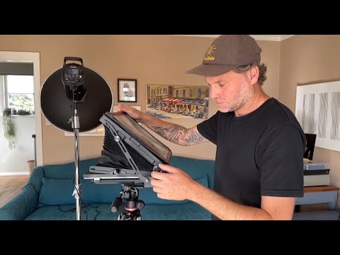
Photography basics: Camera Aspect Ratio, Sensor Size and Depth of Field – resolutions
Read more: Photography basics: Camera Aspect Ratio, Sensor Size and Depth of Field – resolutionshttp://www.shutterangle.com/2012/cinematic-look-aspect-ratio-sensor-size-depth-of-field/
http://www.shutterangle.com/2012/film-video-aspect-ratio-artistic-choice/


-
Composition – These are the basic lighting techniques you need to know for photography and film
Read more: Composition – These are the basic lighting techniques you need to know for photography and film
http://www.diyphotography.net/basic-lighting-techniques-need-know-photography-film/
Amongst the basic techniques, there’s…
1- Side lighting – Literally how it sounds, lighting a subject from the side when they’re faced toward you
2- Rembrandt lighting – Here the light is at around 45 degrees over from the front of the subject, raised and pointing down at 45 degrees
3- Back lighting – Again, how it sounds, lighting a subject from behind. This can help to add drama with silouettes
4- Rim lighting – This produces a light glowing outline around your subject
5- Key light – The main light source, and it’s not necessarily always the brightest light source
6- Fill light – This is used to fill in the shadows and provide detail that would otherwise be blackness
7- Cross lighting – Using two lights placed opposite from each other to light two subjects
-
Photography basics: Depth of Field and composition
Read more: Photography basics: Depth of Field and compositionDepth of field is the range within which focusing is resolved in a photo.
Aperture has a huge affect on to the depth of field.
Changing the f-stops (f/#) of a lens will change aperture and as such the DOF.
f-stops are a just certain number which is telling you the size of the aperture. That’s how f-stop is related to aperture (and DOF).
If you increase f-stops, it will increase DOF, the area in focus (and decrease the aperture). On the other hand, decreasing the f-stop it will decrease DOF (and increase the aperture).
The red cone in the figure is an angular representation of the resolution of the system. Versus the dotted lines, which indicate the aperture coverage. Where the lines of the two cones intersect defines the total range of the depth of field.
This image explains why the longer the depth of field, the greater the range of clarity.


DESIGN


COLOR
-
The Color of Infinite Temperature
Read more: The Color of Infinite TemperatureThis is the color of something infinitely hot.

Of course you’d instantly be fried by gamma rays of arbitrarily high frequency, but this would be its spectrum in the visible range.
johncarlosbaez.wordpress.com/2022/01/16/the-color-of-infinite-temperature/
This is also the color of a typical neutron star. They’re so hot they look the same.
It’s also the color of the early Universe!This was worked out by David Madore.

The color he got is sRGB(148,177,255).
www.htmlcsscolor.com/hex/94B1FFAnd according to the experts who sip latte all day and make up names for colors, this color is called ‘Perano’.
-
FXGuide – ACES 2.0 with ILM’s Alex Fry
Read more: FXGuide – ACES 2.0 with ILM’s Alex Fry
https://draftdocs.acescentral.com/background/whats-new/
ACES 2.0 is the second major release of the components that make up the ACES system. The most significant change is a new suite of rendering transforms whose design was informed by collected feedback and requests from users of ACES 1. The changes aim to improve the appearance of perceived artifacts and to complete previously unfinished components of the system, resulting in a more complete, robust, and consistent product.
Highlights of the key changes in ACES 2.0 are as follows:
- New output transforms, including:
- A less aggressive tone scale
- More intuitive controls to create custom outputs to non-standard displays
- Robust gamut mapping to improve perceptual uniformity
- Improved performance of the inverse transforms
- Enhanced AMF specification
- An updated specification for ACES Transform IDs
- OpenEXR compression recommendations
- Enhanced tools for generating Input Transforms and recommended procedures for characterizing prosumer cameras
- Look Transform Library
- Expanded documentation
Rendering Transform
The most substantial change in ACES 2.0 is a complete redesign of the rendering transform.
ACES 2.0 was built as a unified system, rather than through piecemeal additions. Different deliverable outputs “match” better and making outputs to display setups other than the provided presets is intended to be user-driven. The rendering transforms are less likely to produce undesirable artifacts “out of the box”, which means less time can be spent fixing problematic images and more time making pictures look the way you want.
Key design goals
- Improve consistency of tone scale and provide an easy to use parameter to allow for outputs between preset dynamic ranges
- Minimize hue skews across exposure range in a region of same hue
- Unify for structural consistency across transform type
- Easy to use parameters to create outputs other than the presets
- Robust gamut mapping to improve harsh clipping artifacts
- Fill extents of output code value cube (where appropriate and expected)
- Invertible – not necessarily reversible, but Output > ACES > Output round-trip should be possible
- Accomplish all of the above while maintaining an acceptable “out-of-the box” rendering
- New output transforms, including:
-
Björn Ottosson – How software gets color wrong
Read more: Björn Ottosson – How software gets color wronghttps://bottosson.github.io/posts/colorwrong/
Most software around us today are decent at accurately displaying colors. Processing of colors is another story unfortunately, and is often done badly.
To understand what the problem is, let’s start with an example of three ways of blending green and magenta:
- Perceptual blend – A smooth transition using a model designed to mimic human perception of color. The blending is done so that the perceived brightness and color varies smoothly and evenly.
- Linear blend – A model for blending color based on how light behaves physically. This type of blending can occur in many ways naturally, for example when colors are blended together by focus blur in a camera or when viewing a pattern of two colors at a distance.
- sRGB blend – This is how colors would normally be blended in computer software, using sRGB to represent the colors.

Let’s look at some more examples of blending of colors, to see how these problems surface more practically. The examples use strong colors since then the differences are more pronounced. This is using the same three ways of blending colors as the first example.

Instead of making it as easy as possible to work with color, most software make it unnecessarily hard, by doing image processing with representations not designed for it. Approximating the physical behavior of light with linear RGB models is one easy thing to do, but more work is needed to create image representations tailored for image processing and human perception.
Also see:
-
Tobia Montanari – Memory Colors: an essential tool for Colorists
Read more: Tobia Montanari – Memory Colors: an essential tool for Coloristshttps://www.tobiamontanari.com/memory-colors-an-essential-tool-for-colorists/
“Memory colors are colors that are universally associated with specific objects, elements or scenes in our environment. They are the colors that we expect to see in specific situations: these colors are based on our expectation of how certain objects should look based on our past experiences and memories.
For instance, we associate specific hues, saturation and brightness values with human skintones and a slight variation can significantly affect the way we perceive a scene.
Similarly, we expect blue skies to have a particular hue, green trees to be a specific shade and so on.
Memory colors live inside of our brains and we often impose them onto what we see. By considering them during the grading process, the resulting image will be more visually appealing and won’t distract the viewer from the intended message of the story. Even a slight deviation from memory colors in a movie can create a sense of discordance, ultimately detracting from the viewer’s experience.”


LIGHTING
-
Convert between light exposure and intensity
Read more: Convert between light exposure and intensityimport math,sys def Exposure2Intensity(exposure): exp = float(exposure) result = math.pow(2,exp) print(result) Exposure2Intensity(0) def Intensity2Exposure(intensity): inarg = float(intensity) if inarg == 0: print("Exposure of zero intensity is undefined.") return if inarg < 1e-323: inarg = max(inarg, 1e-323) print("Exposure of negative intensities is undefined. Clamping to a very small value instead (1e-323)") result = math.log(inarg, 2) print(result) Intensity2Exposure(0.1)Why Exposure?
Exposure is a stop value that multiplies the intensity by 2 to the power of the stop. Increasing exposure by 1 results in double the amount of light.
Artists think in “stops.” Doubling or halving brightness is easy math and common in grading and look-dev.
Exposure counts doublings in whole stops:- +1 stop = ×2 brightness
- −1 stop = ×0.5 brightness
This gives perceptually even controls across both bright and dark values.
Why Intensity?
Intensity is linear.
It’s what render engines and compositors expect when:- Summing values
- Averaging pixels
- Multiplying or filtering pixel data
Use intensity when you need the actual math on pixel/light data.
Formulas (from your Python)
- Intensity from exposure: intensity = 2**exposure
- Exposure from intensity: exposure = log₂(intensity)
Guardrails:
- Intensity must be > 0 to compute exposure.
- If intensity = 0 → exposure is undefined.
- Clamp tiny values (e.g.
1e−323) before using log₂.
Use Exposure (stops) when…
- You want artist-friendly sliders (−5…+5 stops)
- Adjusting look-dev or grading in even stops
- Matching plates with quick ±1 stop tweaks
- Tweening brightness changes smoothly across ranges
Use Intensity (linear) when…
- Storing raw pixel/light values
- Multiplying textures or lights by a gain
- Performing sums, averages, and filters
- Feeding values to render engines expecting linear data
Examples
- +2 stops → 2**2 = 4.0 (×4)
- +1 stop → 2**1 = 2.0 (×2)
- 0 stop → 2**0 = 1.0 (×1)
- −1 stop → 2**(−1) = 0.5 (×0.5)
- −2 stops → 2**(−2) = 0.25 (×0.25)
- Intensity 0.1 → exposure = log₂(0.1) ≈ −3.32
Rule of thumb
Think in stops (exposure) for controls and matching.
Compute in linear (intensity) for rendering and math. -
The Color of Infinite Temperature
Read more: The Color of Infinite TemperatureThis is the color of something infinitely hot.
Of course you’d instantly be fried by gamma rays of arbitrarily high frequency, but this would be its spectrum in the visible range.
johncarlosbaez.wordpress.com/2022/01/16/the-color-of-infinite-temperature/
This is also the color of a typical neutron star. They’re so hot they look the same.
It’s also the color of the early Universe!This was worked out by David Madore.
The color he got is sRGB(148,177,255).
www.htmlcsscolor.com/hex/94B1FFAnd according to the experts who sip latte all day and make up names for colors, this color is called ‘Perano’.


COLLECTIONS
| Featured AI
| Design And Composition
| Explore posts
POPULAR SEARCHES
unreal | pipeline | virtual production | free | learn | photoshop | 360 | macro | google | nvidia | resolution | open source | hdri | real-time | photography basics | nuke
FEATURED POSTS
-
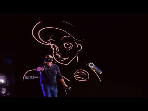
Principles of Animation with Alan Becker, Dermot OConnor and Shaun Keenan
-
copypastecharacter.com – alphabets, special characters, alt codes and symbols library
-
Web vs Printing or digital RGB vs CMYK
-
Convert 2D Images or Text to 3D Models
-
UV maps
-
Decart AI Mirage – The first ever World Transformation Model – turning any video, game, or camera feed into a new digital world, in real time
-
Advanced Computer Vision with Python OpenCV and Mediapipe
-
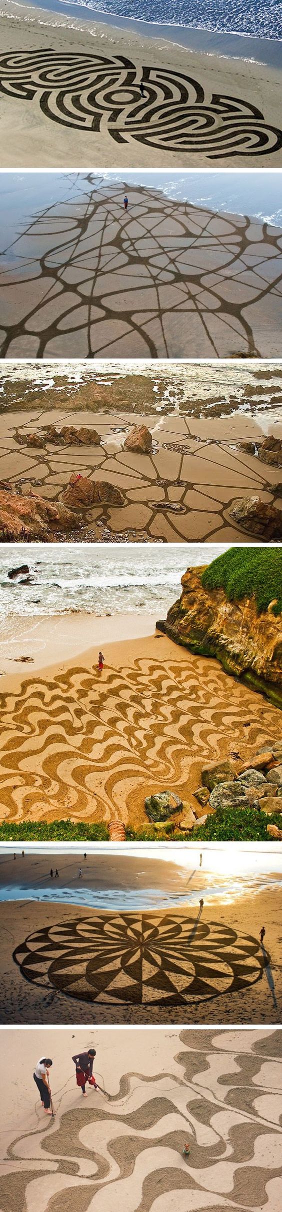
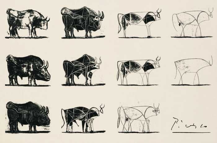
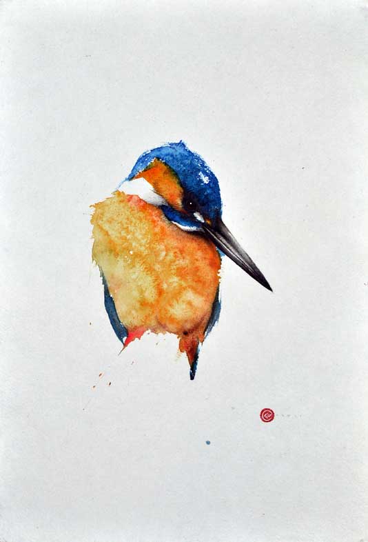
Steven Stahlberg – Perception and Composition
Social Links
DISCLAIMER – Links and images on this website may be protected by the respective owners’ copyright. All data submitted by users through this site shall be treated as freely available to share.
