While the human eye has red, green, and blue-sensing cones, those cones are cross-wired in the retina to produce a luminance channel plus a red-green and a blue-yellow channel, and it’s data in that color space (known technically as “LAB”) that goes to the brain. That’s why we can’t perceive a reddish-green or a yellowish-blue, whereas such colors can be represented in the RGB color space used by digital cameras.
The back of the retina is covered in light-sensitive neurons known as cone cells and rod cells. There are three types of cone cells, each sensitive to different ranges of light. These ranges overlap, but for convenience the cones are referred to as blue (short-wavelength), green (medium-wavelength), and red (long-wavelength). The rod cells are primarily used in low-light situations, so we’ll ignore those for now.
When light enters the eye and hits the cone cells, the cones get excited and send signals to the brain through the visual cortex. Different wavelengths of light excite different combinations of cones to varying levels, which generates our perception of color. You can see that the red cones are most sensitive to light, and the blue cones are least sensitive. The sensitivity of green and red cones overlaps for most of the visible spectrum.
Here’s how your brain takes the signals of light intensity from the cones and turns it into color information. To see red or green, your brain finds the difference between the levels of excitement in your red and green cones. This is the red-green channel.
To get “brightness,” your brain combines the excitement of your red and green cones. This creates the luminance, or black-white, channel. To see yellow or blue, your brain then finds the difference between this luminance signal and the excitement of your blue cones. This is the yellow-blue channel.
From the calculations made in the brain along those three channels, we get four basic colors: blue, green, yellow, and red. Seeing blue is what you experience when low-wavelength light excites the blue cones more than the green and red.
Seeing green happens when light excites the green cones more than the red cones. Seeing red happens when only the red cones are excited by high-wavelength light.
Here’s where it gets interesting. Seeing yellow is what happens when BOTH the green AND red cones are highly excited near their peak sensitivity. This is the biggest collective excitement that your cones ever have, aside from seeing pure white.
Notice that yellow occurs at peak intensity in the graph to the right. Further, the lens and cornea of the eye happen to block shorter wavelengths, reducing sensitivity to blue and violet light.
The Manuka rendering architecture has been designed in the spirit of the classic reyes rendering architecture. In its core, reyes is based on stochastic rasterisation of micropolygons, facilitating depth of field, motion blur, high geometric complexity,and programmable shading.
This is commonly achieved with Monte Carlo path tracing, using a paradigm often called shade-on-hit, in which the renderer alternates tracing rays with running shaders on the various ray hits. The shaders take the role of generating the inputs of the local material structure which is then used bypath sampling logic to evaluate contributions and to inform what further rays to cast through the scene.
Over the years, however, the expectations have risen substantially when it comes to image quality. Computing pictures which are indistinguishable from real footage requires accurate simulation of light transport, which is most often performed using some variant of Monte Carlo path tracing. Unfortunately this paradigm requires random memory accesses to the whole scene and does not lend itself well to a rasterisation approach at all.
Manuka is both a uni-directional and bidirectional path tracer and encompasses multiple importance sampling (MIS). Interestingly, and importantly for production character skin work, it is the first major production renderer to incorporate spectral MIS in the form of a new ‘Hero Spectral Sampling’ technique, which was recently published at Eurographics Symposium on Rendering 2014.
Manuka propose a shade-before-hit paradigm in-stead and minimise I/O strain (and some memory costs) on the system, leveraging locality of reference by running pattern generation shaders before we execute light transport simulation by path sampling, “compressing” any bvh structure as needed, and as such also limiting duplication of source data.
The difference with reyes is that instead of baking colors into the geometry like in Reyes, manuka bakes surface closures. This means that light transport is still calculated with path tracing, but all texture lookups etc. are done up-front and baked into the geometry.
The main drawback with this method is that geometry has to be tessellated to its highest, stable topology before shading can be evaluated properly. As such, the high cost to first pixel. Even a basic 4 vertices square becomes a much more complex model with this approach.
Manuka use the RenderMan Shading Language (rsl) for programmable shading [Pixar Animation Studios 2015], but we do not invoke rsl shaders when intersecting a ray with a surface (often called shade-on-hit). Instead, we pre-tessellate and pre-shade all the input geometry in the front end of the renderer.
This way, we can efficiently order shading computations to sup-port near-optimal texture locality, vectorisation, and parallelism. This system avoids repeated evaluation of shaders at the same surface point, and presents a minimal amount of memory to be accessed during light transport time. An added benefit is that the acceleration structure for ray tracing (abounding volume hierarchy, bvh) is built once on the final tessellated geometry, which allows us to ray trace more efficiently than multi-level bvhs and avoids costly caching of on-demand tessellated micropolygons and the associated scheduling issues.
For the shading reasons above, in terms of AOVs, the studio approach is to succeed at combining complex shading with ray paths in the render rather than pass a multi-pass render to compositing.
For the Spectral Rendering component. The light transport stage is fully spectral, using a continuously sampled wavelength which is traced with each path and used to apply the spectral camera sensitivity of the sensor. This allows for faithfully support any degree of observer metamerism as the camera footage they are intended to match as well as complex materials which require wavelength dependent phenomena such as diffraction, dispersion, interference, iridescence, or chromatic extinction and Rayleigh scattering in participating media.
As opposed to the original reyes paper, we use bilinear interpolation of these bsdf inputs later when evaluating bsdfs per pathv ertex during light transport4. This improves temporal stability of geometry which moves very slowly with respect to the pixel raster
In terms of the pipeline, everything rendered at Weta was already completely interwoven with their deep data pipeline. Manuka very much was written with deep data in mind. Here, Manuka not so much extends the deep capabilities, rather it fully matches the already extremely complex and powerful setup Weta Digital already enjoy with RenderMan. For example, an ape in a scene can be selected, its ID is available and a NUKE artist can then paint in 3D say a hand and part of the way up the neutral posed ape.
We called our system Manuka, as a respectful nod to reyes: we had heard a story froma former ILM employee about how reyes got its name from how fond the early Pixar people were of their lunches at Point Reyes, and decided to name our system after our surrounding natural environment, too. Manuka is a kind of tea tree very common in New Zealand which has very many very small leaves, in analogy to micropolygons ina tree structure for ray tracing. It also happens to be the case that Weta Digital’s main site is on Manuka Street.
In color technology, color depth also known as bit depth, is either the number of bits used to indicate the color of a single pixel, OR the number of bits used for each color component of a single pixel.
When referring to a pixel, the concept can be defined as bits per pixel (bpp).
When referring to a color component, the concept can be defined as bits per component, bits per channel, bits per color (all three abbreviated bpc), and also bits per pixel component, bits per color channel or bits per sample (bps). Modern standards tend to use bits per component, but historical lower-depth systems used bits per pixel more often.
Color depth is only one aspect of color representation, expressing the precision with which the amount of each primary can be expressed; the other aspect is how broad a range of colors can be expressed (the gamut). The definition of both color precision and gamut is accomplished with a color encoding specification which assigns a digital code value to a location in a color space.
“Fix your gaze on the black dot on the left side of this image. But wait! Finish reading this paragraph first. As you gaze at the left dot, try to answer this question: In what direction is the object on the right moving? Is it drifting diagonally, or is it moving up and down?”
Spectralon is a teflon-based pressed powderthat comes closest to being a pure Lambertian diffuse material that reflects 100% of all light. If we take an HDR photograph of the Spectralon alongside the material to be measured, we can derive thediffuse albedo of that material.
The process to capture diffuse reflectance is very similar to the one outlined by Hable.
1. We put a linear polarizing filter in front of the camera lens and a second linear polarizing filterin front of a modeling light or a flash such that the two filters are oriented perpendicular to eachother, i.e. cross polarized.
2. We place Spectralon close to and parallel with the material we are capturing and take brack-eted shots of the setup7. Typically, we’ll take nine photographs, from -4EV to +4EV in 1EVincrements.
3. We convert the bracketed shots to a linear HDR image. We found that many HDR packagesdo not produce an HDR image in which the pixel values are linear. PTGui is an example of apackage which does generate a linear HDR image. At this point, because of the cross polarization,the image is one of surface diffuse response.
4. We open the file in Photoshop and normalize the image by color picking the Spectralon, filling anew layer with that color and setting that layer to “Divide”. This sets the Spectralon to 1 in theimage. All other color values are relative to this so we can consider them as diffuse albedo.
In video terms gamut is normally related to as the full range of colours and brightness that can be either captured or displayed.
Generally speaking all color gamuts recommendations are trying to define a reasonable level of color representation based on available technology and hardware. REC-601 represents the old TVs. REC-709 is currently the most distributed solution. P3 is mainly available in movie theaters and is now being adopted in some of the best new 4K HDR TVs. Rec2020 (a wider space than P3 that improves on visibke color representation) and ACES (the full coverage of visible color) are other common standards which see major hardware development these days.
To compare and visualize different solution (across video and printing solutions), most developers use the CIE color model chart as a reference.
The CIE color model is a color space model created by the International Commission on Illumination known as the Commission Internationale de l’Elcairage (CIE) in 1931. It is also known as the CIE XYZ color space or the CIE 1931 XYZ color space.
This chart represents the first defined quantitative link between distributions of wavelengths in the electromagnetic visible spectrum, and physiologically perceived colors in human color vision. Or basically, the range of color a typical human eye can perceive through visible light.
Note that while the human perception is quite wide, and generally speaking biased towards greens (we are apes after all), the amount of colors available through nature, generated through light reflection, tend to be a much smaller section. This is defined by the Pointer’s Chart.
In short. Color gamut is a representation of color coverage, used to describe data stored in images against available hardware and viewer technologies.
The CIE 1931 standard has been replaced by a CIE 1976 standard. Below we can see the significance of this.
People have observed that the biggest issue with CIE 1931 is the lack of uniformity with chromaticity, the three dimension color space in rectangular coordinates is not visually uniformed.
The CIE 1976 (also called CIELUV) was created by the CIE in 1976. It was put forward in an attempt to provide a more uniform color spacing than CIE 1931 for colors at approximately the same luminance
The CIE 1976 standard colour space is more linear and variations in perceived colour between different people has also been reduced. The disproportionately large green-turquoise area in CIE 1931, which cannot be generated with existing computer screens, has been reduced.
If we move from CIE 1931 to the CIE 1976 standard colour space we can see that the improvements made in the gamut for the “new” iPad screen (as compared to the “old” iPad 2) are more evident in the CIE 1976 colour space than in the CIE 1931 colour space, particularly in the blues from aqua to deep blue.
Despite its age, CIE 1931, named for the year of its adoption, remains a well-worn and familiar shorthand throughout the display industry. CIE 1931 is the primary language of customers. When a customer says that their current display “can do 72% of NTSC,” they implicitly mean 72% of NTSC 1953 color gamut as mapped against CIE 1931.
RGBW (RGB + White) LED strip uses a 4-in-1 LED chip made up of red, green, blue, and white.
RGBWW (RGB + White + Warm White) LED strip uses either a 5-in-1 LED chip with red, green, blue, white, and warm white for color mixing. The only difference between RGBW and RGBWW is the intensity of the white color. The term RGBCCT consists of RGB and CCT. CCT (Correlated Color Temperature) means that the color temperature of the led strip light can be adjusted to change between warm white and white. Thus, RGBWW strip light is another name of RGBCCT strip.
RGBCW is the acronym for Red, Green, Blue, Cold, and Warm. These 5-in-1 chips are used in supper bright smart LED lighting products
Basically, gamma is the relationship between the brightness of a pixel as it appears on the screen, and the numerical value of that pixel. Generally Gamma is just about defining relationships.
Three main types: – Image Gamma encoded in images – Display Gammas encoded in hardware and/or viewing time – System or Viewing Gamma which is the net effect of all gammas when you look back at a final image. In theory this should flatten back to 1.0 gamma.
The intricate relationship between the eyes and the brain, often termed the eye-mind connection, reveals that vision is predominantly a cognitive process. This understanding has profound implications for fields such as design, where capturing and maintaining attention is paramount. This essay delves into the nuances of visual perception, the brain’s role in interpreting visual data, and how this knowledge can be applied to effective design strategies.
This cognitive aspect of vision is evident in phenomena such as optical illusions, where the brain interprets visual information in a way that contradicts physical reality. These illusions underscore that what we “see” is not merely a direct recording of the external world but a constructed experience shaped by cognitive processes.
Understanding the cognitive nature of vision is crucial for effective design. Designers must consider how the brain processes visual information to create compelling and engaging visuals. This involves several key principles:
DISCLAIMER – Links and images on this website may be protected by the respective owners’ copyright. All data submitted by users through this site shall be treated as freely available to share.