In the retina, photoreceptors, bipolar cells, and horizontal cells work together to process visual information before it reaches the brain. Here’s how each cell type contributes to vision:
ACES 2.0 is the second major release of the components that make up the ACES system. The most significant change is a new suite of rendering transforms whose design was informed by collected feedback and requests from users of ACES 1. The changes aim to improve the appearance of perceived artifacts and to complete previously unfinished components of the system, resulting in a more complete, robust, and consistent product.
Highlights of the key changes in ACES 2.0 are as follows:
New output transforms, including:
A less aggressive tone scale
More intuitive controls to create custom outputs to non-standard displays
Robust gamut mapping to improve perceptual uniformity
Improved performance of the inverse transforms
Enhanced AMF specification
An updated specification for ACES Transform IDs
OpenEXR compression recommendations
Enhanced tools for generating Input Transforms and recommended procedures for characterizing prosumer cameras
Look Transform Library
Expanded documentation
Rendering Transform
The most substantial change in ACES 2.0 is a complete redesign of the rendering transform.
ACES 2.0 was built as a unified system, rather than through piecemeal additions. Different deliverable outputs “match” better and making outputs to display setups other than the provided presets is intended to be user-driven. The rendering transforms are less likely to produce undesirable artifacts “out of the box”, which means less time can be spent fixing problematic images and more time making pictures look the way you want.
Key design goals
Improve consistency of tone scale and provide an easy to use parameter to allow for outputs between preset dynamic ranges
Minimize hue skews across exposure range in a region of same hue
Unify for structural consistency across transform type
Easy to use parameters to create outputs other than the presets
Robust gamut mapping to improve harsh clipping artifacts
Fill extents of output code value cube (where appropriate and expected)
Invertible – not necessarily reversible, but Output > ACES > Output round-trip should be possible
Accomplish all of the above while maintaining an acceptable “out-of-the box” rendering
The power output of a light source is measured using the unit of watts W. This is a direct measure to calculate how much power the light is going to drain from your socket and it is not relatable to the light brightness itself.
The amount of energy emitted from it per second. That energy comes out in a form of photons which we can crudely represent with rays of light coming out of the source. The higher the power the more rays emitted from the source in a unit of time.
Not all energy emitted is visible to the human eye, so we often rely on photometric measurements, which takes in account the sensitivity of human eye to different wavelenghts
Divesh Naidoo: The video below was made with a live in-camera preview and auto-exposure matching, no camera solve, no HDRI capture and no manual compositing setup. Using the new Simulon phone app.
import math,sys

def Exposure2Intensity(exposure):
    exp = float(exposure)
    result = math.pow(2,exp)
    print(result)

Exposure2Intensity(0)

def Intensity2Exposure(intensity):
    inarg = float(intensity)

    if inarg == 0:
        print("Exposure of zero intensity is undefined.")
        return

    if inarg < 1e-323:
        inarg = max(inarg, 1e-323)
        print("Exposure of negative intensities is undefined. Clamping to a very small value instead (1e-323)")

    result = math.log(inarg, 2)
    print(result)

Intensity2Exposure(0.1)
Why Exposure?
Exposure is a stop value that multiplies the intensity by 2 to the power of the stop. Increasing exposure by 1 results in double the amount of light.
Artists think in “stops.” Doubling or halving brightness is easy math and common in grading and look-dev. Exposure counts doublings in whole stops:
+1 stop = ×2 brightness
−1 stop = ×0.5 brightness
This gives perceptually even controls across both bright and dark values.
Why Intensity?
Intensity is linear. It’s what render engines and compositors expect when:
Summing values
Averaging pixels
Multiplying or filtering pixel data
Use intensity when you need the actual math on pixel/light data.
Formulas (from your Python)
Intensity from exposure: intensity = 2**exposure
Exposure from intensity: exposure = log₂(intensity)
Guardrails:
Intensity must be > 0 to compute exposure.
If intensity = 0 → exposure is undefined.
Clamp tiny values (e.g. 1e−323) before using log₂.
Use Exposure (stops) when…
You want artist-friendly sliders (−5…+5 stops)
Adjusting look-dev or grading in even stops
Matching plates with quick ±1 stop tweaks
Tweening brightness changes smoothly across ranges
Use Intensity (linear) when…
Storing raw pixel/light values
Multiplying textures or lights by a gain
Performing sums, averages, and filters
Feeding values to render engines expecting linear data
Examples
+2 stops → 2**2 = 4.0 (×4)
+1 stop → 2**1 = 2.0 (×2)
0 stop → 2**0 = 1.0 (×1)
−1 stop → 2**(−1) = 0.5 (×0.5)
−2 stops → 2**(−2) = 0.25 (×0.25)
Intensity 0.1 → exposure = log₂(0.1) ≈ −3.32
Rule of thumb
Think in stops (exposure) for controls and matching. Compute in linear (intensity) for rendering and math.
DISCLAIMER – Links and images on this website may be protected by the respective owners’ copyright. All data submitted by users through this site shall be treated as freely available to share.