This page compares images rendered in Arnold using spectral rendering and different sets of colourspace primaries: Rec.709, Rec.2020, ACES and DCI-P3. The SPD data for the GretagMacbeth Color Checker are the measurements of Noburu Ohta, taken from Mansencal, Mauderer and Parsons (2014) colour-science.org.
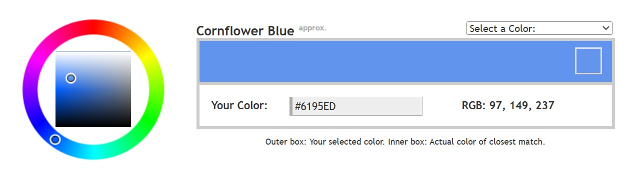
Note: In Foundry’s Nuke, the software will map 18% gray to whatever your center f/stop is set to in the viewer settings (f/8 by default… change that to EV by following the instructions below).
You can experiment with this by attaching an Exposure node to a Constant set to 0.18, setting your viewer read-out to Spotmeter, and adjusting the stops in the node up and down. You will see that a full stop up or down will give you the respective next value on the aperture scale (f8, f11, f16 etc.).
One stop doubles or halves the amount or light that hits the filmback/ccd, so everything works in powers of 2.
So starting with 0.18 in your constant, you will see that raising it by a stop will give you .36 as a floating point number (in linear space), while your f/stop will be f/11 and so on.
If you set your center stop to 0 (see below) you will get a relative readout in EVs, where EV 0 again equals 18% constant gray.
In other words. Setting the center f-stop to 0 means that in a neutral plate, the middle gray in the macbeth chart will equal to exposure value 0. EV 0 corresponds to an exposure time of 1 sec and an aperture of f/1.0.
This will set the sun usually around EV12-17 and the sky EV1-4 , depending on cloud coverage.
To switch Foundry’s Nuke’s SpotMeter to return the EV of an image, click on the main viewport, and then press s, this opens the viewer’s properties. Now set the center f-stop to 0 in there. And the SpotMeter in the viewport will change from aperture and fstops to EV.
The goals of lighting in 3D computer graphics are more or less the same as those of real world lighting.
Lighting serves a basic function of bringing out, or pushing back the shapes of objects visible from the camera’s view.
It gives a two-dimensional image on the monitor an illusion of the third dimension-depth.
But it does not just stop there. It gives an image its personality, its character. A scene lit in different ways can give a feeling of happiness, of sorrow, of fear etc., and it can do so in dramatic or subtle ways. Along with personality and character, lighting fills a scene with emotion that is directly transmitted to the viewer.
Trying to simulate a real environment in an artificial one can be a daunting task. But even if you make your 3D rendering look absolutely photo-realistic, it doesn’t guarantee that the image carries enough emotion to elicit a “wow” from the people viewing it.
Making 3D renderings photo-realistic can be hard. Putting deep emotions in them can be even harder. However, if you plan out your lighting strategy for the mood and emotion that you want your rendering to express, you make the process easier for yourself.
Each light source can be broken down in to 4 distinct components and analyzed accordingly.
· Intensity
· Direction
· Color
· Size
The overall thrust of this writing is to produce photo-realistic images by applying good lighting techniques.
A light wave that is vibrating in more than one plane is referred to as unpolarized light. …
Polarized light waves are light waves in which the vibrations occur in a single plane. The process of transforming unpolarized light into polarized light is known as polarization.
The most common use of polarized technology is to reduce lighting complexity on the subject. Details such as glare and hard edges are not removed, but greatly reduced.
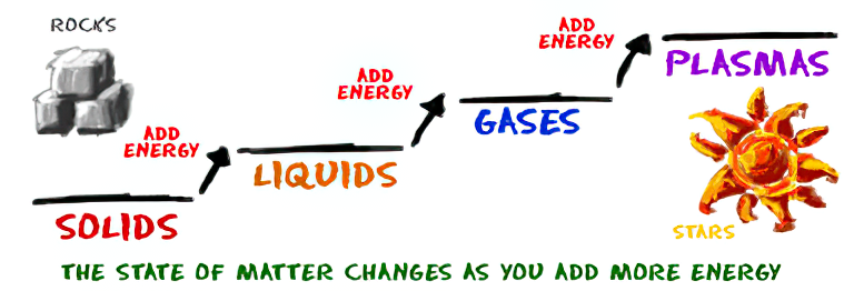
As Einstein showed us, light and matter and just aspects of the same thing. Matter is just frozen light. And light is matter on the move. Albert Einstein’s most famous equation says that energy and matter are two sides of the same coin. How does one become the other?
Relativity requires that the faster an object moves, the more mass it appears to have. This means that somehow part of the energy of the car’s motion appears to transform into mass. Hence the origin of Einstein’s equation. How does that happen? We don’t really know. We only know that it does.
Matter is 99.999999999999 percent empty space. Not only do the atom and solid matter consist mainly of empty space, it is the same in outer space
The quantum theory researchers discovered the answer: Not only do particles consist of energy, but so does the space between. This is the so-called zero-point energy. Therefore it is true: Everything consists of energy.
Energy is the basis of material reality. Every type of particle is conceived of as a quantum vibration in a field: Electrons are vibrations in electron fields, protons vibrate in a proton field, and so on. Everything is energy, and everything is connected to everything else through fields.
In photography, exposure value (EV) is a number that represents a combination of a camera’s shutter speed and f-number, such that all combinations that yield the same exposure have the same EV (for any fixed scene luminance).
The EV concept was developed in an attempt to simplify choosing among combinations of equivalent camera settings. Although all camera settings with the same EV nominally give the same exposure, they do not necessarily give the same picture. EV is also used to indicate an interval on the photographic exposure scale. 1 EV corresponding to a standard power-of-2 exposure step, commonly referred to as a stop
EV 0 corresponds to an exposure time of 1 sec and a relative aperture of f/1.0. If the EV is known, it can be used to select combinations of exposure time and f-number.
Note EV does not equal to photographic exposure. Photographic Exposureis defined as how much light hits the camera’s sensor. It depends on the camera settings mainly aperture and shutter speed. Exposure value (known as EV) is a number that represents theexposure setting of the camera.
Thus, strictly, EV is not a measure of luminance (indirect or reflected exposure) or illuminance (incidentl exposure); rather, an EV corresponds to a luminance (or illuminance) for which a camera with a given ISO speed would use the indicated EV to obtain the nominally correct exposure. Nonetheless, it is common practice among photographic equipment manufacturers to express luminance in EV for ISO 100 speed, as when specifying metering range or autofocus sensitivity.
The exposure depends on two things: how much light gets through the lenses to the camera’s sensor and for how long the sensor is exposed. The former is a function of the aperture value while the latter is a function of the shutter speed. Exposure value is a number that represents this potential amount of light that could hit the sensor. It is important to understand that exposure value is a measure of how exposed the sensor is to light and not a measure of how much light actually hits the sensor. The exposure value is independent of how lit the scene is. For example a pair of aperture value and shutter speed represents the same exposure value both if the camera is used during a very bright day or during a dark night.
Each exposure value number represents all the possible shutter and aperture settings that result in the same exposure. Although the exposure value is the same for different combinations of aperture values and shutter speeds the resulting photo can be very different (the aperture controls the depth of field while shutter speed controls how much motion is captured).
EV 0.0 is defined as the exposure when setting the aperture to f-number 1.0 and the shutter speed to 1 second. All other exposure values are relative to that number. Exposure values are on a base two logarithmic scale. This means that every single step of EV – plus or minus 1 – represents the exposure (actual light that hits the sensor) being halved or doubled.
If you have no previous experience with Unity, start with these six video tutorials which give a quick overview of the Unity interface and some important features http://unity3d.com/support/documentation/video/
Divesh Naidoo: The video below was made with a live in-camera preview and auto-exposure matching, no camera solve, no HDRI capture and no manual compositing setup. Using the new Simulon phone app.
To measure the contrast ratio you will need a light meter. The process starts with you measuring the main source of light, or the key light.
Get a reading from the brightest area on the face of your subject. Then, measure the area lit by the secondary light, or fill light. To make sense of what you have just measured you have to understand that the information you have just gathered is in F-stops, a measure of light. With each additional F-stop, for example going one stop from f/1.4 to f/2.0, you create a doubling of light. The reverse is also true; moving one stop from f/8.0 to f/5.6 results in a halving of the light.
IES profiles are useful for creating life-like lighting, as they can represent the physical distribution of light from any light source.
The IES format was created by the Illumination Engineering Society, and most lighting manufacturers provide IES profile for the lights they manufacture.
DISCLAIMER – Links and images on this website may be protected by the respective owners’ copyright. All data submitted by users through this site shall be treated as freely available to share.