


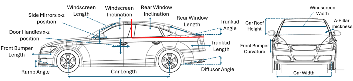
COMPOSITION


DESIGN
-
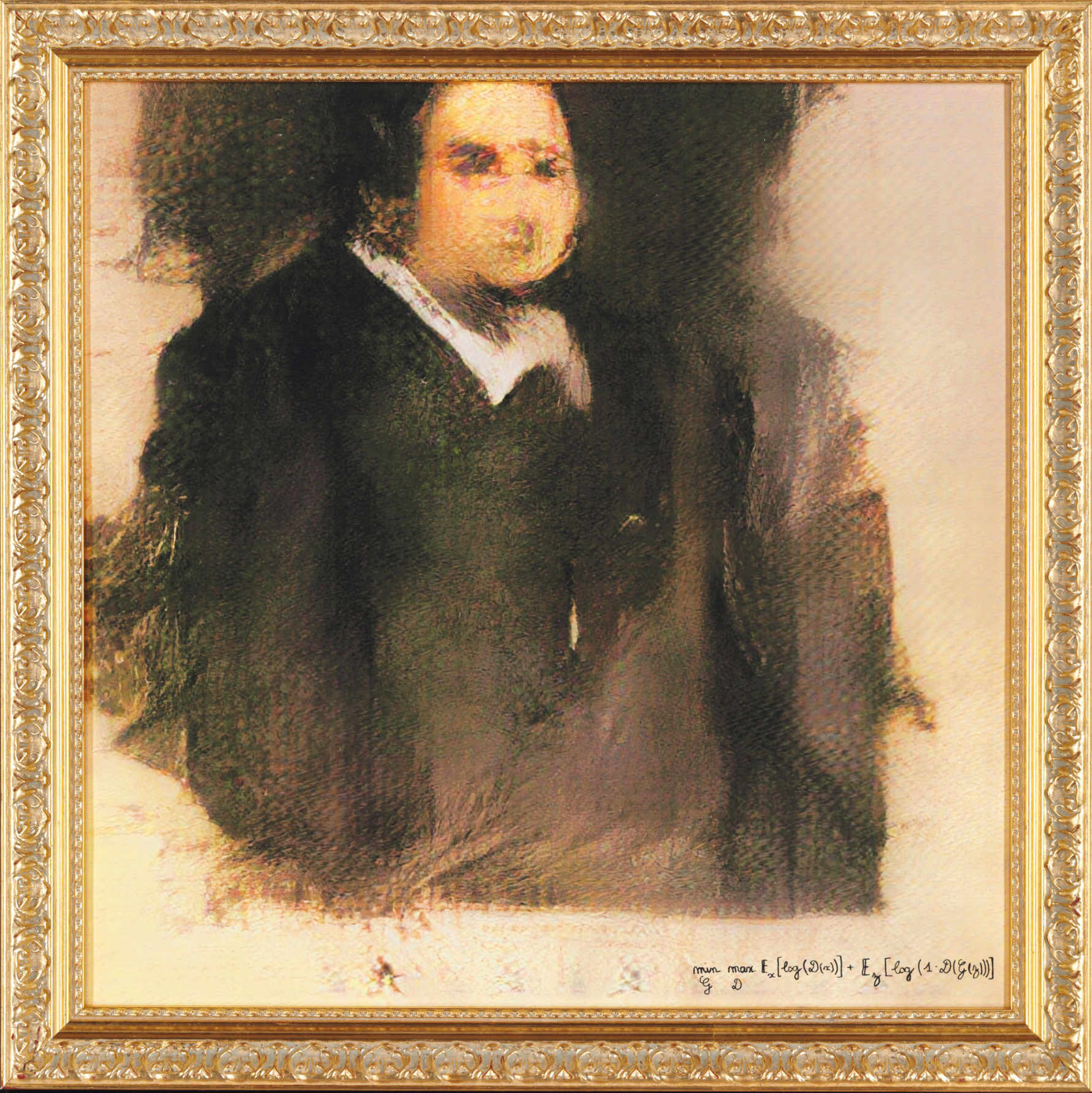
A.I. Algorithm art fetches US$432,500 at Christie auction
Read more: A.I. Algorithm art fetches US$432,500 at Christie auctionwww.ctvnews.ca/entertainment/algorithm-art-fetches-us-432-500-at-christie-s-auction-1.4150620
www.christies.com/features/A-collaboration-between-two-artists-one-human-one-a-machine-9332-1.aspx


COLOR
-
mmColorTarget – Nuke Gizmo for color matching a MacBeth chart
Read more: mmColorTarget – Nuke Gizmo for color matching a MacBeth charthttps://www.marcomeyer-vfx.de/posts/2014-04-11-mmcolortarget-nuke-gizmo/
https://www.marcomeyer-vfx.de/posts/mmcolortarget-nuke-gizmo/
https://vimeo.com/9.1652466e+07
https://www.nukepedia.com/gizmos/colour/mmcolortarget
-
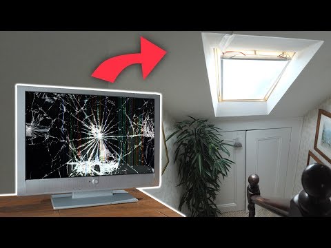
OLED vs QLED – What TV is better?
Read more: OLED vs QLED – What TV is better?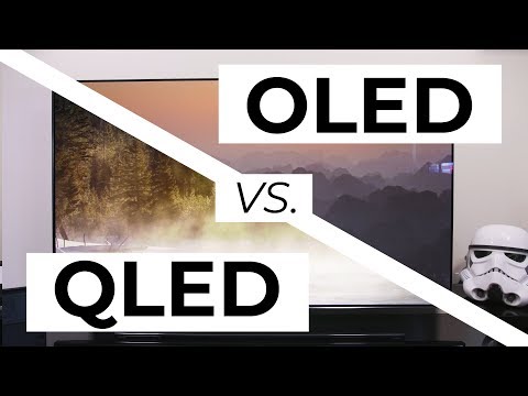
Supported by LG, Philips, Panasonic and Sony sell the OLED system TVs.
OLED stands for “organic light emitting diode.”
It is a fundamentally different technology from LCD, the major type of TV today.
OLED is “emissive,” meaning the pixels emit their own light.Samsung is branding its best TVs with a new acronym: “QLED”
QLED (according to Samsung) stands for “quantum dot LED TV.”
It is a variation of the common LED LCD, adding a quantum dot film to the LCD “sandwich.”
QLED, like LCD, is, in its current form, “transmissive” and relies on an LED backlight.OLED is the only technology capable of absolute blacks and extremely bright whites on a per-pixel basis. LCD definitely can’t do that, and even the vaunted, beloved, dearly departed plasma couldn’t do absolute blacks.
QLED, as an improvement over OLED, significantly improves the picture quality. QLED can produce an even wider range of colors than OLED, which says something about this new tech. QLED is also known to produce up to 40% higher luminance efficiency than OLED technology. Further, many tests conclude that QLED is far more efficient in terms of power consumption than its predecessor, OLED.
(more…) -
GretagMacbeth Color Checker Numeric Values and Middle Gray
Read more: GretagMacbeth Color Checker Numeric Values and Middle GrayThe human eye perceives half scene brightness not as the linear 50% of the present energy (linear nature values) but as 18% of the overall brightness. We are biased to perceive more information in the dark and contrast areas. A Macbeth chart helps with calibrating back into a photographic capture into this “human perspective” of the world.
https://en.wikipedia.org/wiki/Middle_gray
In photography, painting, and other visual arts, middle gray or middle grey is a tone that is perceptually about halfway between black and white on a lightness scale in photography and printing, it is typically defined as 18% reflectance in visible light

Light meters, cameras, and pictures are often calibrated using an 18% gray card[4][5][6] or a color reference card such as a ColorChecker. On the assumption that 18% is similar to the average reflectance of a scene, a grey card can be used to estimate the required exposure of the film.
https://en.wikipedia.org/wiki/ColorChecker
(more…) -
The Maya civilization and the color blue
Read more: The Maya civilization and the color blueMaya blue is a highly unusual pigment because it is a mix of organic indigo and an inorganic clay mineral called palygorskite.
Echoing the color of an azure sky, the indelible pigment was used to accentuate everything from ceramics to human sacrifices in the Late Preclassic period (300 B.C. to A.D. 300).
A team of researchers led by Dean Arnold, an adjunct curator of anthropology at the Field Museum in Chicago, determined that the key to Maya blue was actually a sacred incense called copal.
By heating the mixture of indigo, copal and palygorskite over a fire, the Maya produced the unique pigment, he reported at the time.
-
PTGui 13 beta adds control through a Patch Editor
Read more: PTGui 13 beta adds control through a Patch EditorAdditions:
- Patch Editor (PTGui Pro)
- DNG output
- Improved RAW / DNG handling
- JPEG 2000 support
- Performance improvements


LIGHTING
-
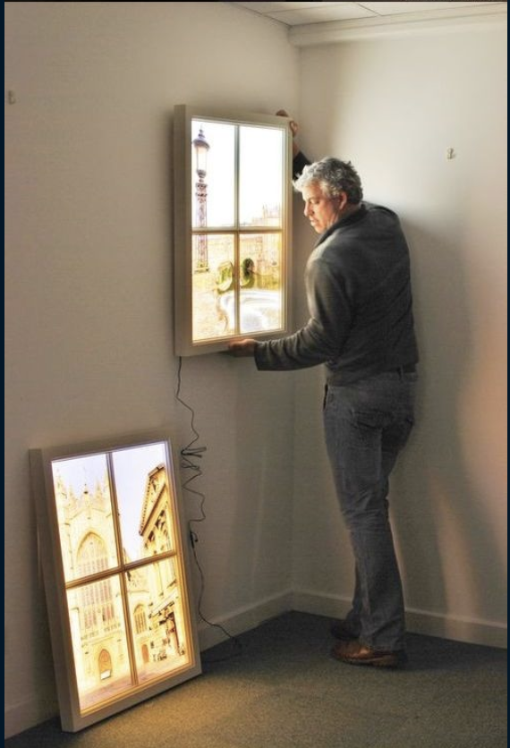
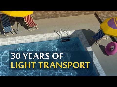
Capturing the world in HDR for real time projects – Call of Duty: Advanced Warfare
Read more: Capturing the world in HDR for real time projects – Call of Duty: Advanced WarfareReal-World Measurements for Call of Duty: Advanced Warfare
www.activision.com/cdn/research/Real_World_Measurements_for_Call_of_Duty_Advanced_Warfare.pdf
Local version
Real_World_Measurements_for_Call_of_Duty_Advanced_Warfare.pdf

-
Romain Chauliac – LightIt a lighting script for Maya and Arnold
Read more: Romain Chauliac – LightIt a lighting script for Maya and ArnoldLightIt is a script for Maya and Arnold that will help you and improve your lighting workflow.
Thanks to preset studio lighting components (lights, backdrop…), high quality studio scenes and HDRI library manager.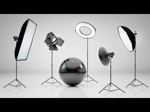
https://www.artstation.com/artwork/393emJ


COLLECTIONS
| Featured AI
| Design And Composition
| Explore posts
POPULAR SEARCHES
unreal | pipeline | virtual production | free | learn | photoshop | 360 | macro | google | nvidia | resolution | open source | hdri | real-time | photography basics | nuke
FEATURED POSTS
-
Top 3D Printing Website Resources
-
What Is The Resolution and view coverage Of The human Eye. And what distance is TV at best?
-
Survivorship Bias: The error resulting from systematically focusing on successes and ignoring failures. How a young statistician saved his planes during WW2.
-
Tencent Hunyuan3D 2.1 goes Open Source and adds MV (Multi-view) and MV Mini
-
Ross Pettit on The Agile Manager – How tech firms went for prioritizing cash flow instead of talent (and artists)
-
Film Production walk-through – pipeline – I want to make a … movie
-
Kling 1.6 and competitors – advanced tests and comparisons
-
GretagMacbeth Color Checker Numeric Values and Middle Gray
Social Links
DISCLAIMER – Links and images on this website may be protected by the respective owners’ copyright. All data submitted by users through this site shall be treated as freely available to share.
