Depth of field is the range within which focusing is resolved in a photo.
Aperture has a huge affect on to the depth of field.
Changing the f-stops (f/#) of a lens will change aperture and as such the DOF.
f-stops are a just certain number which is telling you the size of the aperture. That’s how f-stop is related to aperture (and DOF).
If you increase f-stops, it will increase DOF, the area in focus (and decrease the aperture). On the other hand, decreasing the f-stop it will decrease DOF (and increase the aperture).
The red cone in the figure is an angular representation of the resolution of the system. Versus the dotted lines, which indicate the aperture coverage. Where the lines of the two cones intersect defines the total range of the depth of field.
This image explains why the longer the depth of field, the greater the range of clarity.
Hand drawn sketch | Models made in CC4 with ZBrush | Textures in Substance Painter | Paint over in Photoshop | Renders, Animation, VFX with AI. Each 5-8 hours spread over a couple days.
As I continue to explore the use of AI tools to enhance my 3D character creation process, I discover they can be incredibly useful during the previsualization phase to see what a character might ultimately look like in production. I selectively use AI to enhance and accelerate my creative process, not to replace it or use it as an end to end solution.
Spectral sensitivity of eye is influenced by light intensity. And the light intensity determines the level of activity of cones cell and rod cell. This is the main characteristic of human vision. Sensitivity to individual colors, in other words, wavelengths of the light spectrum, is explained by the RGB (red-green-blue) theory. This theory assumed that there are three kinds of cones. It’s selectively sensitive to red (700-630 nm), green (560-500 nm), and blue (490-450 nm) light. And their mutual interaction allow to perceive all colors of the spectrum.
While the human eye has red, green, and blue-sensing cones, those cones are cross-wired in the retina to produce a luminance channel plus a red-green and a blue-yellow channel, and it’s data in that color space (known technically as “LAB”) that goes to the brain. That’s why we can’t perceive a reddish-green or a yellowish-blue, whereas such colors can be represented in the RGB color space used by digital cameras.
The back of the retina is covered in light-sensitive neurons known as cone cells and rod cells. There are three types of cone cells, each sensitive to different ranges of light. These ranges overlap, but for convenience the cones are referred to as blue (short-wavelength), green (medium-wavelength), and red (long-wavelength). The rod cells are primarily used in low-light situations, so we’ll ignore those for now.
When light enters the eye and hits the cone cells, the cones get excited and send signals to the brain through the visual cortex. Different wavelengths of light excite different combinations of cones to varying levels, which generates our perception of color. You can see that the red cones are most sensitive to light, and the blue cones are least sensitive. The sensitivity of green and red cones overlaps for most of the visible spectrum.
Here’s how your brain takes the signals of light intensity from the cones and turns it into color information. To see red or green, your brain finds the difference between the levels of excitement in your red and green cones. This is the red-green channel.
To get “brightness,” your brain combines the excitement of your red and green cones. This creates the luminance, or black-white, channel. To see yellow or blue, your brain then finds the difference between this luminance signal and the excitement of your blue cones. This is the yellow-blue channel.
From the calculations made in the brain along those three channels, we get four basic colors: blue, green, yellow, and red. Seeing blue is what you experience when low-wavelength light excites the blue cones more than the green and red.
Seeing green happens when light excites the green cones more than the red cones. Seeing red happens when only the red cones are excited by high-wavelength light.
Here’s where it gets interesting. Seeing yellow is what happens when BOTH the green AND red cones are highly excited near their peak sensitivity. This is the biggest collective excitement that your cones ever have, aside from seeing pure white.
Notice that yellow occurs at peak intensity in the graph to the right. Further, the lens and cornea of the eye happen to block shorter wavelengths, reducing sensitivity to blue and violet light.
The human eye perceives half scene brightness not as the linear 50% of the present energy (linear nature values) but as 18% of the overall brightness. We are biased to perceive more information in the dark and contrast areas. A Macbeth chart helps with calibrating back into a photographic capture into this “human perspective” of the world.
In photography, painting, and other visual arts, middle gray or middle grey is a tone that is perceptually about halfway between black and white on a lightness scale in photography and printing, it is typically defined as 18% reflectance in visible light
Light meters, cameras, and pictures are often calibrated using an 18% gray card[4][5][6] or a color reference card such as a ColorChecker. On the assumption that 18% is similar to the average reflectance of a scene, a grey card can be used to estimate the required exposure of the film.
The power output of a light source is measured using the unit of watts W. This is a direct measure to calculate how much power the light is going to drain from your socket and it is not relatable to the light brightness itself.
The amount of energy emitted from it per second. That energy comes out in a form of photons which we can crudely represent with rays of light coming out of the source. The higher the power the more rays emitted from the source in a unit of time.
Not all energy emitted is visible to the human eye, so we often rely on photometric measurements, which takes in account the sensitivity of human eye to different wavelenghts
The Manuka rendering architecture has been designed in the spirit of the classic reyes rendering architecture. In its core, reyes is based on stochastic rasterisation of micropolygons, facilitating depth of field, motion blur, high geometric complexity,and programmable shading.
This is commonly achieved with Monte Carlo path tracing, using a paradigm often called shade-on-hit, in which the renderer alternates tracing rays with running shaders on the various ray hits. The shaders take the role of generating the inputs of the local material structure which is then used bypath sampling logic to evaluate contributions and to inform what further rays to cast through the scene.
Over the years, however, the expectations have risen substantially when it comes to image quality. Computing pictures which are indistinguishable from real footage requires accurate simulation of light transport, which is most often performed using some variant of Monte Carlo path tracing. Unfortunately this paradigm requires random memory accesses to the whole scene and does not lend itself well to a rasterisation approach at all.
Manuka is both a uni-directional and bidirectional path tracer and encompasses multiple importance sampling (MIS). Interestingly, and importantly for production character skin work, it is the first major production renderer to incorporate spectral MIS in the form of a new ‘Hero Spectral Sampling’ technique, which was recently published at Eurographics Symposium on Rendering 2014.
Manuka propose a shade-before-hit paradigm in-stead and minimise I/O strain (and some memory costs) on the system, leveraging locality of reference by running pattern generation shaders before we execute light transport simulation by path sampling, “compressing” any bvh structure as needed, and as such also limiting duplication of source data.
The difference with reyes is that instead of baking colors into the geometry like in Reyes, manuka bakes surface closures. This means that light transport is still calculated with path tracing, but all texture lookups etc. are done up-front and baked into the geometry.
The main drawback with this method is that geometry has to be tessellated to its highest, stable topology before shading can be evaluated properly. As such, the high cost to first pixel. Even a basic 4 vertices square becomes a much more complex model with this approach.
Manuka use the RenderMan Shading Language (rsl) for programmable shading [Pixar Animation Studios 2015], but we do not invoke rsl shaders when intersecting a ray with a surface (often called shade-on-hit). Instead, we pre-tessellate and pre-shade all the input geometry in the front end of the renderer.
This way, we can efficiently order shading computations to sup-port near-optimal texture locality, vectorisation, and parallelism. This system avoids repeated evaluation of shaders at the same surface point, and presents a minimal amount of memory to be accessed during light transport time. An added benefit is that the acceleration structure for ray tracing (abounding volume hierarchy, bvh) is built once on the final tessellated geometry, which allows us to ray trace more efficiently than multi-level bvhs and avoids costly caching of on-demand tessellated micropolygons and the associated scheduling issues.
For the shading reasons above, in terms of AOVs, the studio approach is to succeed at combining complex shading with ray paths in the render rather than pass a multi-pass render to compositing.
For the Spectral Rendering component. The light transport stage is fully spectral, using a continuously sampled wavelength which is traced with each path and used to apply the spectral camera sensitivity of the sensor. This allows for faithfully support any degree of observer metamerism as the camera footage they are intended to match as well as complex materials which require wavelength dependent phenomena such as diffraction, dispersion, interference, iridescence, or chromatic extinction and Rayleigh scattering in participating media.
As opposed to the original reyes paper, we use bilinear interpolation of these bsdf inputs later when evaluating bsdfs per pathv ertex during light transport4. This improves temporal stability of geometry which moves very slowly with respect to the pixel raster
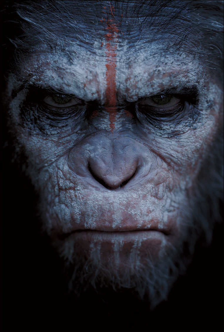
In terms of the pipeline, everything rendered at Weta was already completely interwoven with their deep data pipeline. Manuka very much was written with deep data in mind. Here, Manuka not so much extends the deep capabilities, rather it fully matches the already extremely complex and powerful setup Weta Digital already enjoy with RenderMan. For example, an ape in a scene can be selected, its ID is available and a NUKE artist can then paint in 3D say a hand and part of the way up the neutral posed ape.
We called our system Manuka, as a respectful nod to reyes: we had heard a story froma former ILM employee about how reyes got its name from how fond the early Pixar people were of their lunches at Point Reyes, and decided to name our system after our surrounding natural environment, too. Manuka is a kind of tea tree very common in New Zealand which has very many very small leaves, in analogy to micropolygons ina tree structure for ray tracing. It also happens to be the case that Weta Digital’s main site is on Manuka Street.
Basically, gamma is the relationship between the brightness of a pixel as it appears on the screen, and the numerical value of that pixel. Generally Gamma is just about defining relationships.
Three main types: – Image Gamma encoded in images – Display Gammas encoded in hardware and/or viewing time – System or Viewing Gamma which is the net effect of all gammas when you look back at a final image. In theory this should flatten back to 1.0 gamma.
When collecting hdri make sure the data supports basic metadata, such as:
Iso
Aperture
Exposure time or shutter time
Color temperature
Color space Exposure value (what the sensor receives of the sun intensity in lux)
7+ brackets (with 5 or 6 being the perceived balanced exposure)
In image processing, computer graphics, and photography, high dynamic range imaging (HDRI or just HDR) is a set of techniques that allow a greater dynamic range of luminances (a Photometry measure of the luminous intensity per unit area of light travelling in a given direction. It describes the amount of light that passes through or is emitted from a particular area, and falls within a given solid angle) between the lightest and darkest areas of an image than standard digital imaging techniques or photographic methods. This wider dynamic range allows HDR images to represent more accurately the wide range of intensity levels found in real scenes ranging from direct sunlight to faint starlight and to the deepest shadows.
The two main sources of HDR imagery are computer renderings and merging of multiple photographs, which in turn are known as low dynamic range (LDR) or standard dynamic range (SDR) images. Tone Mapping (Look-up) techniques, which reduce overall contrast to facilitate display of HDR images on devices with lower dynamic range, can be applied to produce images with preserved or exaggerated local contrast for artistic effect. Photography
In photography, dynamic range is measured in Exposure Values (in photography, exposure value denotes all combinations of camera shutter speed and relative aperture that give the same exposure. The concept was developed in Germany in the 1950s) differences or stops, between the brightest and darkest parts of the image that show detail. An increase of one EV or one stop is a doubling of the amount of light.
The human response to brightness is well approximated by a Steven’s power law, which over a reasonable range is close to logarithmic, as described by the Weber�Fechner law, which is one reason that logarithmic measures of light intensity are often used as well.
HDR is short for High Dynamic Range. It’s a term used to describe an image which contains a greater exposure range than the “black” to “white” that 8 or 16-bit integer formats (JPEG, TIFF, PNG) can describe. Whereas these Low Dynamic Range images (LDR) can hold perhaps 8 to 10 f-stops of image information, HDR images can describe beyond 30 stops and stored in 32 bit images.
Ethan Roffler I recently had the honor of interviewing this VFX genius and gained great insight into what it takes to work in the entertainment industry. Keep in mind, these questions are coming from an artist’s perspective but can be applied to any creative individual looking for some wisdom from a professional. So grab a drink, sit back, and enjoy this fun and insightful conversation.
Ethan To start, I just wanted to say thank you so much for taking the time for this interview!
Daniele My pleasure. When I started my career I struggled to find help. Even people in the industry at the time were not that helpful. Because of that, I decided very early on that I was going to do exactly the opposite. I spend most of my weekends talking or helping students. ;)
Ethan That’s awesome! I have also come across the same struggle! Just a heads up, this will probably be the most informal interview you’ll ever have haha! Okay, so let’s start with a small introduction!
An exposure stop is a unit measurement of Exposure as such it provides a universal linear scale to measure the increase and decrease in light, exposed to the image sensor, due to changes in shutter speed, iso and f-stop.
+-1 stop is a doubling or halving of the amount of light let in when taking a photo
1 EV (exposure value) is just another way to say one stop of exposure change.
Same applies to shutter speed, iso and aperture.
Doubling or halving your shutter speed produces an increase or decrease of 1 stop of exposure.
Doubling or halving your iso speed produces an increase or decrease of 1 stop of exposure.
DISCLAIMER – Links and images on this website may be protected by the respective owners’ copyright. All data submitted by users through this site shall be treated as freely available to share.


