


COMPOSITION
DESIGN


COLOR
-
The Forbidden colors – Red-Green & Blue-Yellow: The Stunning Colors You Can’t See
Read more: The Forbidden colors – Red-Green & Blue-Yellow: The Stunning Colors You Can’t Seewww.livescience.com/17948-red-green-blue-yellow-stunning-colors.html

While the human eye has red, green, and blue-sensing cones, those cones are cross-wired in the retina to produce a luminance channel plus a red-green and a blue-yellow channel, and it’s data in that color space (known technically as “LAB”) that goes to the brain. That’s why we can’t perceive a reddish-green or a yellowish-blue, whereas such colors can be represented in the RGB color space used by digital cameras.
https://en.rockcontent.com/blog/the-use-of-yellow-in-data-design
The back of the retina is covered in light-sensitive neurons known as cone cells and rod cells. There are three types of cone cells, each sensitive to different ranges of light. These ranges overlap, but for convenience the cones are referred to as blue (short-wavelength), green (medium-wavelength), and red (long-wavelength). The rod cells are primarily used in low-light situations, so we’ll ignore those for now.
When light enters the eye and hits the cone cells, the cones get excited and send signals to the brain through the visual cortex. Different wavelengths of light excite different combinations of cones to varying levels, which generates our perception of color. You can see that the red cones are most sensitive to light, and the blue cones are least sensitive. The sensitivity of green and red cones overlaps for most of the visible spectrum.

Here’s how your brain takes the signals of light intensity from the cones and turns it into color information. To see red or green, your brain finds the difference between the levels of excitement in your red and green cones. This is the red-green channel.
To get “brightness,” your brain combines the excitement of your red and green cones. This creates the luminance, or black-white, channel. To see yellow or blue, your brain then finds the difference between this luminance signal and the excitement of your blue cones. This is the yellow-blue channel.
From the calculations made in the brain along those three channels, we get four basic colors: blue, green, yellow, and red. Seeing blue is what you experience when low-wavelength light excites the blue cones more than the green and red.
Seeing green happens when light excites the green cones more than the red cones. Seeing red happens when only the red cones are excited by high-wavelength light.
Here’s where it gets interesting. Seeing yellow is what happens when BOTH the green AND red cones are highly excited near their peak sensitivity. This is the biggest collective excitement that your cones ever have, aside from seeing pure white.
Notice that yellow occurs at peak intensity in the graph to the right. Further, the lens and cornea of the eye happen to block shorter wavelengths, reducing sensitivity to blue and violet light.
-
Björn Ottosson – How software gets color wrong
Read more: Björn Ottosson – How software gets color wronghttps://bottosson.github.io/posts/colorwrong/
Most software around us today are decent at accurately displaying colors. Processing of colors is another story unfortunately, and is often done badly.
To understand what the problem is, let’s start with an example of three ways of blending green and magenta:
- Perceptual blend – A smooth transition using a model designed to mimic human perception of color. The blending is done so that the perceived brightness and color varies smoothly and evenly.
- Linear blend – A model for blending color based on how light behaves physically. This type of blending can occur in many ways naturally, for example when colors are blended together by focus blur in a camera or when viewing a pattern of two colors at a distance.
- sRGB blend – This is how colors would normally be blended in computer software, using sRGB to represent the colors.

Let’s look at some more examples of blending of colors, to see how these problems surface more practically. The examples use strong colors since then the differences are more pronounced. This is using the same three ways of blending colors as the first example.

Instead of making it as easy as possible to work with color, most software make it unnecessarily hard, by doing image processing with representations not designed for it. Approximating the physical behavior of light with linear RGB models is one easy thing to do, but more work is needed to create image representations tailored for image processing and human perception.
Also see:
-
FXGuide – ACES 2.0 with ILM’s Alex Fry
Read more: FXGuide – ACES 2.0 with ILM’s Alex Fry
https://draftdocs.acescentral.com/background/whats-new/
ACES 2.0 is the second major release of the components that make up the ACES system. The most significant change is a new suite of rendering transforms whose design was informed by collected feedback and requests from users of ACES 1. The changes aim to improve the appearance of perceived artifacts and to complete previously unfinished components of the system, resulting in a more complete, robust, and consistent product.
Highlights of the key changes in ACES 2.0 are as follows:
- New output transforms, including:
- A less aggressive tone scale
- More intuitive controls to create custom outputs to non-standard displays
- Robust gamut mapping to improve perceptual uniformity
- Improved performance of the inverse transforms
- Enhanced AMF specification
- An updated specification for ACES Transform IDs
- OpenEXR compression recommendations
- Enhanced tools for generating Input Transforms and recommended procedures for characterizing prosumer cameras
- Look Transform Library
- Expanded documentation
Rendering Transform
The most substantial change in ACES 2.0 is a complete redesign of the rendering transform.
ACES 2.0 was built as a unified system, rather than through piecemeal additions. Different deliverable outputs “match” better and making outputs to display setups other than the provided presets is intended to be user-driven. The rendering transforms are less likely to produce undesirable artifacts “out of the box”, which means less time can be spent fixing problematic images and more time making pictures look the way you want.
Key design goals
- Improve consistency of tone scale and provide an easy to use parameter to allow for outputs between preset dynamic ranges
- Minimize hue skews across exposure range in a region of same hue
- Unify for structural consistency across transform type
- Easy to use parameters to create outputs other than the presets
- Robust gamut mapping to improve harsh clipping artifacts
- Fill extents of output code value cube (where appropriate and expected)
- Invertible – not necessarily reversible, but Output > ACES > Output round-trip should be possible
- Accomplish all of the above while maintaining an acceptable “out-of-the box” rendering
- New output transforms, including:
-
SecretWeapons MixBox – a practical library for paint-like digital color mixing
Read more: SecretWeapons MixBox – a practical library for paint-like digital color mixingInternally, Mixbox treats colors as real-life pigments using the Kubelka & Munk theory to predict realistic color behavior.
https://scrtwpns.com/mixbox/painter/
https://scrtwpns.com/mixbox.pdf
https://github.com/scrtwpns/mixbox
https://scrtwpns.com/mixbox/docs/

-
Paul Debevec, Chloe LeGendre, Lukas Lepicovsky – Jointly Optimizing Color Rendition and In-Camera Backgrounds in an RGB Virtual Production Stage
Read more: Paul Debevec, Chloe LeGendre, Lukas Lepicovsky – Jointly Optimizing Color Rendition and In-Camera Backgrounds in an RGB Virtual Production Stagehttps://arxiv.org/pdf/2205.12403.pdf
RGB LEDs vs RGBWP (RGB + lime + phospor converted amber) LEDs
Local copy:
-
Rec-2020 – TVs new color gamut standard used by Dolby Vision?
Read more: Rec-2020 – TVs new color gamut standard used by Dolby Vision?https://www.hdrsoft.com/resources/dri.html#bit-depth

The dynamic range is a ratio between the maximum and minimum values of a physical measurement. Its definition depends on what the dynamic range refers to.
For a scene: Dynamic range is the ratio between the brightest and darkest parts of the scene.
For a camera: Dynamic range is the ratio of saturation to noise. More specifically, the ratio of the intensity that just saturates the camera to the intensity that just lifts the camera response one standard deviation above camera noise.
For a display: Dynamic range is the ratio between the maximum and minimum intensities emitted from the screen.
The Dynamic Range of real-world scenes can be quite high — ratios of 100,000:1 are common in the natural world. An HDR (High Dynamic Range) image stores pixel values that span the whole tonal range of real-world scenes. Therefore, an HDR image is encoded in a format that allows the largest range of values, e.g. floating-point values stored with 32 bits per color channel. Another characteristics of an HDR image is that it stores linear values. This means that the value of a pixel from an HDR image is proportional to the amount of light measured by the camera.
For TVs HDR is great, but it’s not the only new TV feature worth discussing.
(more…) -
Black Body color aka the Planckian Locus curve for white point eye perception
Read more: Black Body color aka the Planckian Locus curve for white point eye perceptionhttp://en.wikipedia.org/wiki/Black-body_radiation

Black-body radiation is the type of electromagnetic radiation within or surrounding a body in thermodynamic equilibrium with its environment, or emitted by a black body (an opaque and non-reflective body) held at constant, uniform temperature. The radiation has a specific spectrum and intensity that depends only on the temperature of the body.
A black-body at room temperature appears black, as most of the energy it radiates is infra-red and cannot be perceived by the human eye. At higher temperatures, black bodies glow with increasing intensity and colors that range from dull red to blindingly brilliant blue-white as the temperature increases.
(more…)


LIGHTING
-
Rendering – BRDF – Bidirectional reflectance distribution function
Read more: Rendering – BRDF – Bidirectional reflectance distribution functionhttp://en.wikipedia.org/wiki/Bidirectional_reflectance_distribution_function
The bidirectional reflectance distribution function is a four-dimensional function that defines how light is reflected at an opaque surface
http://www.cs.ucla.edu/~zhu/tutorial/An_Introduction_to_BRDF-Based_Lighting.pdf
In general, when light interacts with matter, a complicated light-matter dynamic occurs. This interaction depends on the physical characteristics of the light as well as the physical composition and characteristics of the matter.
That is, some of the incident light is reflected, some of the light is transmitted, and another portion of the light is absorbed by the medium itself.
A BRDF describes how much light is reflected when light makes contact with a certain material. Similarly, a BTDF (Bi-directional Transmission Distribution Function) describes how much light is transmitted when light makes contact with a certain material
http://www.cs.princeton.edu/~smr/cs348c-97/surveypaper.html
It is difficult to establish exactly how far one should go in elaborating the surface model. A truly complete representation of the reflective behavior of a surface might take into account such phenomena as polarization, scattering, fluorescence, and phosphorescence, all of which might vary with position on the surface. Therefore, the variables in this complete function would be:
incoming and outgoing angle incoming and outgoing wavelength incoming and outgoing polarization (both linear and circular) incoming and outgoing position (which might differ due to subsurface scattering) time delay between the incoming and outgoing light ray
-
Fast, optimized ‘for’ pixel loops with OpenCV and Python to create tone mapped HDR images
Read more: Fast, optimized ‘for’ pixel loops with OpenCV and Python to create tone mapped HDR imageshttps://pyimagesearch.com/2017/08/28/fast-optimized-for-pixel-loops-with-opencv-and-python/
https://learnopencv.com/exposure-fusion-using-opencv-cpp-python/
Exposure Fusion is a method for combining images taken with different exposure settings into one image that looks like a tone mapped High Dynamic Range (HDR) image.

-
HDRI shooting and editing by Xuan Prada and Greg Zaal
Read more: HDRI shooting and editing by Xuan Prada and Greg Zaalwww.xuanprada.com/blog/2014/11/3/hdri-shooting
http://blog.gregzaal.com/2016/03/16/make-your-own-hdri/
http://blog.hdrihaven.com/how-to-create-high-quality-hdri/
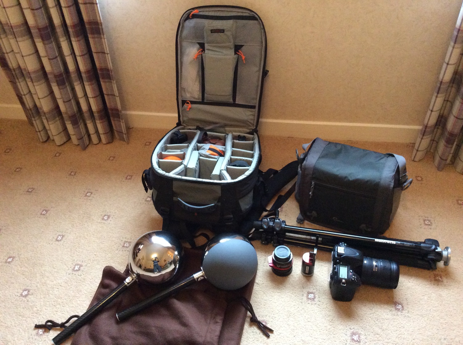
Shooting checklist
- Full coverage of the scene (fish-eye shots)
- Backplates for look-development (including ground or floor)
- Macbeth chart for white balance
- Grey ball for lighting calibration
- Chrome ball for lighting orientation
- Basic scene measurements
- Material samples
- Individual HDR artificial lighting sources if required
Methodology
(more…) -
Convert between light exposure and intensity
Read more: Convert between light exposure and intensityimport math,sys def Exposure2Intensity(exposure): exp = float(exposure) result = math.pow(2,exp) print(result) Exposure2Intensity(0) def Intensity2Exposure(intensity): inarg = float(intensity) if inarg == 0: print("Exposure of zero intensity is undefined.") return if inarg < 1e-323: inarg = max(inarg, 1e-323) print("Exposure of negative intensities is undefined. Clamping to a very small value instead (1e-323)") result = math.log(inarg, 2) print(result) Intensity2Exposure(0.1)Why Exposure?
Exposure is a stop value that multiplies the intensity by 2 to the power of the stop. Increasing exposure by 1 results in double the amount of light.
Artists think in “stops.” Doubling or halving brightness is easy math and common in grading and look-dev.
Exposure counts doublings in whole stops:- +1 stop = ×2 brightness
- −1 stop = ×0.5 brightness
This gives perceptually even controls across both bright and dark values.
Why Intensity?
Intensity is linear.
It’s what render engines and compositors expect when:- Summing values
- Averaging pixels
- Multiplying or filtering pixel data
Use intensity when you need the actual math on pixel/light data.
Formulas (from your Python)
- Intensity from exposure: intensity = 2**exposure
- Exposure from intensity: exposure = log₂(intensity)
Guardrails:
- Intensity must be > 0 to compute exposure.
- If intensity = 0 → exposure is undefined.
- Clamp tiny values (e.g.
1e−323) before using log₂.
Use Exposure (stops) when…
- You want artist-friendly sliders (−5…+5 stops)
- Adjusting look-dev or grading in even stops
- Matching plates with quick ±1 stop tweaks
- Tweening brightness changes smoothly across ranges
Use Intensity (linear) when…
- Storing raw pixel/light values
- Multiplying textures or lights by a gain
- Performing sums, averages, and filters
- Feeding values to render engines expecting linear data
Examples
- +2 stops → 2**2 = 4.0 (×4)
- +1 stop → 2**1 = 2.0 (×2)
- 0 stop → 2**0 = 1.0 (×1)
- −1 stop → 2**(−1) = 0.5 (×0.5)
- −2 stops → 2**(−2) = 0.25 (×0.25)
- Intensity 0.1 → exposure = log₂(0.1) ≈ −3.32
Rule of thumb
Think in stops (exposure) for controls and matching.
Compute in linear (intensity) for rendering and math. -
Magnific.ai Relight – change the entire lighting of a scene
Read more: Magnific.ai Relight – change the entire lighting of a scene
It’s a new Magnific spell that allows you to change the entire lighting of a scene and, optionally, the background with just:
1/ A prompt OR
2/ A reference image OR
3/ A light map (drawing your own lights)https://x.com/javilopen/status/1805274155065176489


-
PTGui 13 beta adds control through a Patch Editor
Read more: PTGui 13 beta adds control through a Patch EditorAdditions:
- Patch Editor (PTGui Pro)
- DNG output
- Improved RAW / DNG handling
- JPEG 2000 support
- Performance improvements


COLLECTIONS
| Featured AI
| Design And Composition
| Explore posts
POPULAR SEARCHES
unreal | pipeline | virtual production | free | learn | photoshop | 360 | macro | google | nvidia | resolution | open source | hdri | real-time | photography basics | nuke
FEATURED POSTS
Social Links
DISCLAIMER – Links and images on this website may be protected by the respective owners’ copyright. All data submitted by users through this site shall be treated as freely available to share.
