slowmoVideo is an OpenSource program that creates slow-motion videos from your footage.
Slow motion cinematography is the result of playing back frames for a longer duration than they were exposed. For example, if you expose 240 frames of film in one second, then play them back at 24 fps, the resulting movie is 10 times longer (slower) than the original filmed event….
Film cameras are relatively simple mechanical devices that allow you to crank up the speed to whatever rate the shutter and pull-down mechanism allow. Some film cameras can operate at 2,500 fps or higher (although film shot in these cameras often needs some readjustment in postproduction). Video, on the other hand, is always captured, recorded, and played back at a fixed rate, with a current limit around 60fps. This makes extreme slow motion effects harder to achieve (and less elegant) on video, because slowing down the video results in each frame held still on the screen for a long time, whereas with high-frame-rate film there are plenty of frames to fill the longer durations of time. On video, the slow motion effect is more like a slide show than smooth, continuous motion.
One obvious solution is to shoot film at high speed, then transfer it to video (a case where film still has a clear advantage, sorry George). Another possibility is to cross dissolve or blur from one frame to the next. This adds a smooth transition from one still frame to the next. The blur reduces the sharpness of the image, and compared to slowing down images shot at a high frame rate, this is somewhat of a cheat. However, there isn’t much you can do about it until video can be recorded at much higher rates. Of course, many film cameras can’t shoot at high frame rates either, so the whole super-slow-motion endeavor is somewhat specialized no matter what medium you are using. (There are some high speed digital cameras available now that allow you to capture lots of digital frames directly to your computer, so technology is starting to catch up with film. However, this feature isn’t going to appear in consumer camcorders any time soon.)
The way humans see the world… until we have a way to describe something, even something so fundamental as a colour, we may not even notice that something it’s there.
Ancient languages didn’t have a word for blue — not Greek, not Chinese, not Japanese, not Hebrew, not Icelandic cultures. And without a word for the colour, there’s evidence that they may not have seen it at all. https://www.wnycstudios.org/story/211119-colors
Every language first had a word for black and for white, or dark and light. The next word for a colour to come into existence — in every language studied around the world — was red, the colour of blood and wine. After red, historically, yellow appears, and later, green (though in a couple of languages, yellow and green switch places). The last of these colours to appear in every language is blue.
The only ancient culture to develop a word for blue was the Egyptians — and as it happens, they were also the only culture that had a way to produce a blue dye. https://mymodernmet.com/shades-of-blue-color-history/
True blue hues are rare in the natural world because synthesizing pigments that absorb longer-wavelength light (reds and yellows) while reflecting shorter-wavelength blue light requires exceptionally elaborate molecular structures—biochemical feats that most plants and animals simply don’t undertake.
When you gaze at a blueberry’s deep blue surface, you’re actually seeing structural coloration rather than a true blue pigment. A fine, waxy bloom on the berry’s skin contains nanostructures that preferentially scatter blue and violet light, giving the fruit its signature blue sheen even though its inherent pigment is reddish.
Similarly, many of nature’s most striking blues—like those of blue jays and morpho butterflies—arise not from blue pigments but from microscopic architectures in feathers or wing scales. These tiny ridges and air pockets manipulate incoming light so that blue wavelengths emerge most prominently, creating vivid, angle-dependent colors through scattering rather than pigment alone.
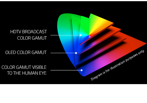
OLED stands for Organic Light Emitting Diode. Each pixel in an OLED display is made of a material that glows when you jab it with electricity. Kind of like the heating elements in a toaster, but with less heat and better resolution. This effect is called electroluminescence, which is one of those delightful words that is big, but actually makes sense: “electro” for electricity, “lumin” for light and “escence” for, well, basically “essence.”
OLED TV marketing often claims “infinite” contrast ratios, and while that might sound like typical hyperbole, it’s one of the extremely rare instances where such claims are actually true. Since OLED can produce a perfect black, emitting no light whatsoever, its contrast ratio (expressed as the brightest white divided by the darkest black) is technically infinite.
OLED is the only technology capable of absolute blacks and extremely bright whites on a per-pixel basis. LCD definitely can’t do that, and even the vaunted, beloved, dearly departed plasma couldn’t do absolute blacks.
ACES 2.0 is the second major release of the components that make up the ACES system. The most significant change is a new suite of rendering transforms whose design was informed by collected feedback and requests from users of ACES 1. The changes aim to improve the appearance of perceived artifacts and to complete previously unfinished components of the system, resulting in a more complete, robust, and consistent product.
Highlights of the key changes in ACES 2.0 are as follows:
New output transforms, including:
A less aggressive tone scale
More intuitive controls to create custom outputs to non-standard displays
Robust gamut mapping to improve perceptual uniformity
Improved performance of the inverse transforms
Enhanced AMF specification
An updated specification for ACES Transform IDs
OpenEXR compression recommendations
Enhanced tools for generating Input Transforms and recommended procedures for characterizing prosumer cameras
Look Transform Library
Expanded documentation
Rendering Transform
The most substantial change in ACES 2.0 is a complete redesign of the rendering transform.
ACES 2.0 was built as a unified system, rather than through piecemeal additions. Different deliverable outputs “match” better and making outputs to display setups other than the provided presets is intended to be user-driven. The rendering transforms are less likely to produce undesirable artifacts “out of the box”, which means less time can be spent fixing problematic images and more time making pictures look the way you want.
Key design goals
Improve consistency of tone scale and provide an easy to use parameter to allow for outputs between preset dynamic ranges
Minimize hue skews across exposure range in a region of same hue
Unify for structural consistency across transform type
Easy to use parameters to create outputs other than the presets
Robust gamut mapping to improve harsh clipping artifacts
Fill extents of output code value cube (where appropriate and expected)
Invertible – not necessarily reversible, but Output > ACES > Output round-trip should be possible
Accomplish all of the above while maintaining an acceptable “out-of-the box” rendering
A LUT (Lookup Table) is essentially the modifier between two images, the original image and the displayed image, based on a mathematical formula. Basically conversion matrices of different complexities. There are different types of LUTS – viewing, transform, calibration, 1D and 3D.
Spectral sensitivity of eye is influenced by light intensity. And the light intensity determines the level of activity of cones cell and rod cell. This is the main characteristic of human vision. Sensitivity to individual colors, in other words, wavelengths of the light spectrum, is explained by the RGB (red-green-blue) theory. This theory assumed that there are three kinds of cones. It’s selectively sensitive to red (700-630 nm), green (560-500 nm), and blue (490-450 nm) light. And their mutual interaction allow to perceive all colors of the spectrum.
By stimulating specific cells in the retina, the participants claim to have witnessed a blue-green colour that scientists have called “olo”, but some experts have said the existence of a new colour is “open to argument”.
The findings, published in the journal Science Advances on Friday, have been described by the study’s co-author, Prof Ren Ng from the University of California, as “remarkable”.
(A) System inputs. (i) Retina map of 103 cone cells preclassified by spectral type (7). (ii) Target visual percept (here, a video of a child, see movie S1 at 1:04). (iii) Infrared cellular-scale imaging of the retina with 60-frames-per-second rolling shutter. Fixational eye movement is visible over the three frames shown.
(B) System outputs. (iv) Real-time per-cone target activation levels to reproduce the target percept, computed by: extracting eye motion from the input video relative to the retina map; identifying the spectral type of every cone in the field of view; computing the per-cone activation the target percept would have produced. (v) Intensities of visible-wavelength 488-nm laser microdoses at each cone required to achieve its target activation level.
(C) Infrared imaging and visible-wavelength stimulation are physically accomplished in a raster scan across the retinal region using AOSLO. By modulating the visible-wavelength beam’s intensity, the laser microdoses shown in (v) are delivered. Drawing adapted with permission [Harmening and Sincich (54)].
(D) Examples of target percepts with corresponding cone activations and laser microdoses, ranging from colored squares to complex imagery. Teal-striped regions represent the color “olo” of stimulating only M cones.
OpenColorIO (OCIO) is a new open source project from Sony Imageworks.
Based on development started in 2003, OCIO enables color transforms and image display to be handled in a consistent manner across multiple graphics applications. Unlike other color management solutions, OCIO is geared towards motion-picture post production, with an emphasis on visual effects and animation color pipelines.
The Manuka rendering architecture has been designed in the spirit of the classic reyes rendering architecture. In its core, reyes is based on stochastic rasterisation of micropolygons, facilitating depth of field, motion blur, high geometric complexity,and programmable shading.
This is commonly achieved with Monte Carlo path tracing, using a paradigm often called shade-on-hit, in which the renderer alternates tracing rays with running shaders on the various ray hits. The shaders take the role of generating the inputs of the local material structure which is then used bypath sampling logic to evaluate contributions and to inform what further rays to cast through the scene.
Over the years, however, the expectations have risen substantially when it comes to image quality. Computing pictures which are indistinguishable from real footage requires accurate simulation of light transport, which is most often performed using some variant of Monte Carlo path tracing. Unfortunately this paradigm requires random memory accesses to the whole scene and does not lend itself well to a rasterisation approach at all.
Manuka is both a uni-directional and bidirectional path tracer and encompasses multiple importance sampling (MIS). Interestingly, and importantly for production character skin work, it is the first major production renderer to incorporate spectral MIS in the form of a new ‘Hero Spectral Sampling’ technique, which was recently published at Eurographics Symposium on Rendering 2014.
Manuka propose a shade-before-hit paradigm in-stead and minimise I/O strain (and some memory costs) on the system, leveraging locality of reference by running pattern generation shaders before we execute light transport simulation by path sampling, “compressing” any bvh structure as needed, and as such also limiting duplication of source data.
The difference with reyes is that instead of baking colors into the geometry like in Reyes, manuka bakes surface closures. This means that light transport is still calculated with path tracing, but all texture lookups etc. are done up-front and baked into the geometry.
The main drawback with this method is that geometry has to be tessellated to its highest, stable topology before shading can be evaluated properly. As such, the high cost to first pixel. Even a basic 4 vertices square becomes a much more complex model with this approach.
Manuka use the RenderMan Shading Language (rsl) for programmable shading [Pixar Animation Studios 2015], but we do not invoke rsl shaders when intersecting a ray with a surface (often called shade-on-hit). Instead, we pre-tessellate and pre-shade all the input geometry in the front end of the renderer.
This way, we can efficiently order shading computations to sup-port near-optimal texture locality, vectorisation, and parallelism. This system avoids repeated evaluation of shaders at the same surface point, and presents a minimal amount of memory to be accessed during light transport time. An added benefit is that the acceleration structure for ray tracing (abounding volume hierarchy, bvh) is built once on the final tessellated geometry, which allows us to ray trace more efficiently than multi-level bvhs and avoids costly caching of on-demand tessellated micropolygons and the associated scheduling issues.
For the shading reasons above, in terms of AOVs, the studio approach is to succeed at combining complex shading with ray paths in the render rather than pass a multi-pass render to compositing.
For the Spectral Rendering component. The light transport stage is fully spectral, using a continuously sampled wavelength which is traced with each path and used to apply the spectral camera sensitivity of the sensor. This allows for faithfully support any degree of observer metamerism as the camera footage they are intended to match as well as complex materials which require wavelength dependent phenomena such as diffraction, dispersion, interference, iridescence, or chromatic extinction and Rayleigh scattering in participating media.
As opposed to the original reyes paper, we use bilinear interpolation of these bsdf inputs later when evaluating bsdfs per pathv ertex during light transport4. This improves temporal stability of geometry which moves very slowly with respect to the pixel raster
In terms of the pipeline, everything rendered at Weta was already completely interwoven with their deep data pipeline. Manuka very much was written with deep data in mind. Here, Manuka not so much extends the deep capabilities, rather it fully matches the already extremely complex and powerful setup Weta Digital already enjoy with RenderMan. For example, an ape in a scene can be selected, its ID is available and a NUKE artist can then paint in 3D say a hand and part of the way up the neutral posed ape.
We called our system Manuka, as a respectful nod to reyes: we had heard a story froma former ILM employee about how reyes got its name from how fond the early Pixar people were of their lunches at Point Reyes, and decided to name our system after our surrounding natural environment, too. Manuka is a kind of tea tree very common in New Zealand which has very many very small leaves, in analogy to micropolygons ina tree structure for ray tracing. It also happens to be the case that Weta Digital’s main site is on Manuka Street.
1 to 100% Stepless Dimming, 1500 Lux Brightness at 3.3′
LCD Info Screen. Powered by an L-series battery, D-Tap, or USB-C
Because the light has a variable color range of 3200 to 9500K, when the light is set to 5500K (daylight balanced) both sets of LEDs are on at full, providing the maximum brightness from this fixture when compared to using the light at 3200 or 9500K.
The LCD screen provides information on the fixture’s output as well as the charge state of the battery. The screen also indicates whether the adjustment knob is controlling brightness or color temperature. To switch from brightness to CCT or CCT to brightness, just apply a short press to the adjustment knob.
The included cold shoe ball joint adapter enables mounting the light to your camera’s accessory shoe via the 1/4″-20 threaded hole on the fixture. In addition, the bottom of the cold shoe foot features a 3/8″-16 threaded hole, and includes a 3/8″-16 to 1/4″-20 reducing bushing.
The intricate relationship between the eyes and the brain, often termed the eye-mind connection, reveals that vision is predominantly a cognitive process. This understanding has profound implications for fields such as design, where capturing and maintaining attention is paramount. This essay delves into the nuances of visual perception, the brain’s role in interpreting visual data, and how this knowledge can be applied to effective design strategies.
This cognitive aspect of vision is evident in phenomena such as optical illusions, where the brain interprets visual information in a way that contradicts physical reality. These illusions underscore that what we “see” is not merely a direct recording of the external world but a constructed experience shaped by cognitive processes.
Understanding the cognitive nature of vision is crucial for effective design. Designers must consider how the brain processes visual information to create compelling and engaging visuals. This involves several key principles:
DISCLAIMER – Links and images on this website may be protected by the respective owners’ copyright. All data submitted by users through this site shall be treated as freely available to share.


 Local copy:


