


COMPOSITION
-
Mastering Camera Shots and Angles: A Guide for Filmmakers
Read more: Mastering Camera Shots and Angles: A Guide for Filmmakershttps://website.ltx.studio/blog/mastering-camera-shots-and-angles
1. Extreme Wide Shot

2. Wide Shot

3. Medium Shot

4. Close Up

5. Extreme Close Up


DESIGN
-
Magic Carpet by artist Daniel Wurtzel
Read more: Magic Carpet by artist Daniel Wurtzelhttps://www.youtube.com/watch?v=1C_40B9m4tI http://www.danielwurtzel.com


COLOR
-
Black Body color aka the Planckian Locus curve for white point eye perception
Read more: Black Body color aka the Planckian Locus curve for white point eye perceptionhttp://en.wikipedia.org/wiki/Black-body_radiation

Black-body radiation is the type of electromagnetic radiation within or surrounding a body in thermodynamic equilibrium with its environment, or emitted by a black body (an opaque and non-reflective body) held at constant, uniform temperature. The radiation has a specific spectrum and intensity that depends only on the temperature of the body.
A black-body at room temperature appears black, as most of the energy it radiates is infra-red and cannot be perceived by the human eye. At higher temperatures, black bodies glow with increasing intensity and colors that range from dull red to blindingly brilliant blue-white as the temperature increases.
(more…) -
Polarised vs unpolarized filtering
Read more: Polarised vs unpolarized filteringA light wave that is vibrating in more than one plane is referred to as unpolarized light. …
Polarized light waves are light waves in which the vibrations occur in a single plane. The process of transforming unpolarized light into polarized light is known as polarization.

en.wikipedia.org/wiki/Polarizing_filter_(photography)
The most common use of polarized technology is to reduce lighting complexity on the subject.
(more…)
Details such as glare and hard edges are not removed, but greatly reduced. -
Tim Kang – calibrated white light values in sRGB color space
Read more: Tim Kang – calibrated white light values in sRGB color space8bit sRGB encoded
2000K 255 139 22
2700K 255 172 89
3000K 255 184 109
3200K 255 190 122
4000K 255 211 165
4300K 255 219 178
D50 255 235 205
D55 255 243 224
D5600 255 244 227
D6000 255 249 240
D65 255 255 255
D10000 202 221 255
D20000 166 196 2558bit Rec709 Gamma 2.4
2000K 255 145 34
2700K 255 177 97
3000K 255 187 117
3200K 255 193 129
4000K 255 214 170
4300K 255 221 182
D50 255 236 208
D55 255 243 226
D5600 255 245 229
D6000 255 250 241
D65 255 255 255
D10000 204 222 255
D20000 170 199 2558bit Display P3 encoded
2000K 255 154 63
2700K 255 185 109
3000K 255 195 127
3200K 255 201 138
4000K 255 219 176
4300K 255 225 187
D50 255 239 212
D55 255 245 228
D5600 255 246 231
D6000 255 251 242
D65 255 255 255
D10000 208 223 255
D20000 175 199 25510bit Rec2020 PQ (100 nits)
2000K 520 435 273
2700K 520 466 358
3000K 520 475 384
3200K 520 480 399
4000K 520 495 446
4300K 520 500 458
D50 520 510 482
D55 520 514 497
D5600 520 514 500
D6000 520 517 509
D65 520 520 520
D10000 479 489 520
D20000 448 464 520
-
Victor Perez – ACES Color Management in DaVinci Resolve
Read more: Victor Perez – ACES Color Management in DaVinci Resolvehttpv://www.youtube.com/watch?v=i–TS88-6xA
-
Scientists claim to have discovered ‘new colour’ no one has seen before: Olo
Read more: Scientists claim to have discovered ‘new colour’ no one has seen before: Olohttps://www.bbc.com/news/articles/clyq0n3em41o
By stimulating specific cells in the retina, the participants claim to have witnessed a blue-green colour that scientists have called “olo”, but some experts have said the existence of a new colour is “open to argument”.
The findings, published in the journal Science Advances on Friday, have been described by the study’s co-author, Prof Ren Ng from the University of California, as “remarkable”.

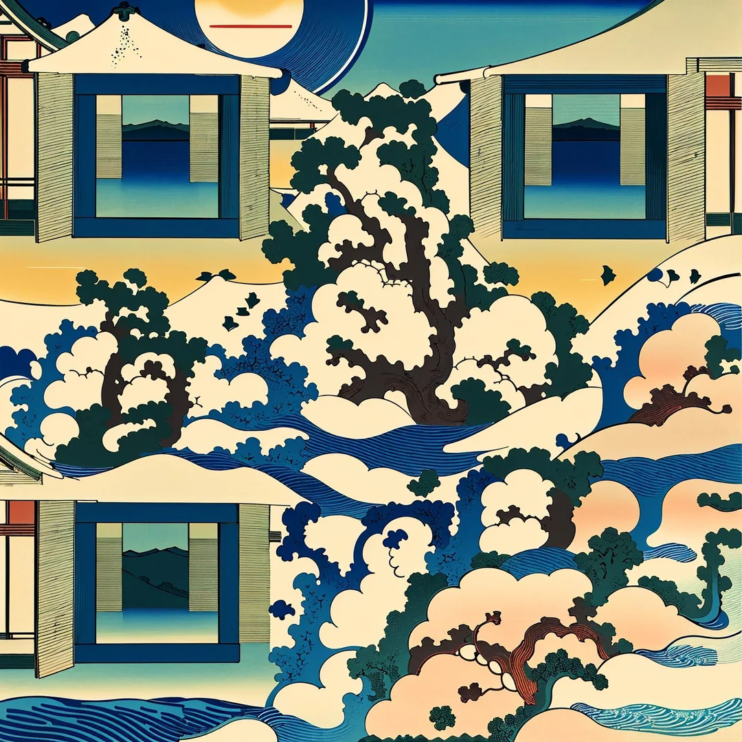
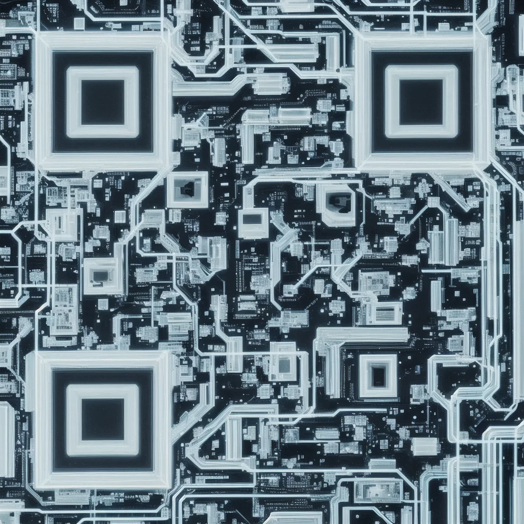
(A) System inputs. (i) Retina map of 103 cone cells preclassified by spectral type (7). (ii) Target visual percept (here, a video of a child, see movie S1 at 1:04). (iii) Infrared cellular-scale imaging of the retina with 60-frames-per-second rolling shutter. Fixational eye movement is visible over the three frames shown.
(B) System outputs. (iv) Real-time per-cone target activation levels to reproduce the target percept, computed by: extracting eye motion from the input video relative to the retina map; identifying the spectral type of every cone in the field of view; computing the per-cone activation the target percept would have produced. (v) Intensities of visible-wavelength 488-nm laser microdoses at each cone required to achieve its target activation level.
(C) Infrared imaging and visible-wavelength stimulation are physically accomplished in a raster scan across the retinal region using AOSLO. By modulating the visible-wavelength beam’s intensity, the laser microdoses shown in (v) are delivered. Drawing adapted with permission [Harmening and Sincich (54)].
(D) Examples of target percepts with corresponding cone activations and laser microdoses, ranging from colored squares to complex imagery. Teal-striped regions represent the color “olo” of stimulating only M cones.
-
Colormaxxing – What if I told you that rgb(255, 0, 0) is not actually the reddest red you can have in your browser?
Read more: Colormaxxing – What if I told you that rgb(255, 0, 0) is not actually the reddest red you can have in your browser?https://karuna.dev/colormaxxing
https://webkit.org/blog-files/color-gamut/comparison.html
https://oklch.com/#70,0.1,197,100
-
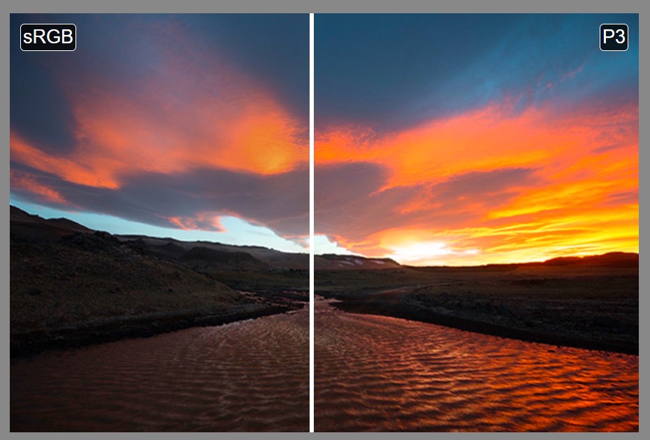
sRGB vs REC709 – An introduction and FFmpeg implementations
Read more: sRGB vs REC709 – An introduction and FFmpeg implementations
1. Basic Comparison
- What they are
- sRGB: A standard “web”/computer-display RGB color space defined by IEC 61966-2-1. It’s used for most monitors, cameras, printers, and the vast majority of images on the Internet.
- Rec. 709: An HD-video color space defined by ITU-R BT.709. It’s the go-to standard for HDTV broadcasts, Blu-ray discs, and professional video pipelines.
- Why they exist
- sRGB: Ensures consistent colors across different consumer devices (PCs, phones, webcams).
- Rec. 709: Ensures consistent colors across video production and playback chains (cameras → editing → broadcast → TV).
- What you’ll see
- On your desktop or phone, images tagged sRGB will look “right” without extra tweaking.
- On an HDTV or video-editing timeline, footage tagged Rec. 709 will display accurate contrast and hue on broadcast-grade monitors.
2. Digging Deeper
Feature sRGB Rec. 709 White point D65 (6504 K), same for both D65 (6504 K) Primaries (x,y) R: (0.640, 0.330) G: (0.300, 0.600) B: (0.150, 0.060) R: (0.640, 0.330) G: (0.300, 0.600) B: (0.150, 0.060) Gamut size Identical triangle on CIE 1931 chart Identical to sRGB Gamma / transfer Piecewise curve: approximate 2.2 with linear toe Pure power-law γ≈2.4 (often approximated as 2.2 in practice) Matrix coefficients N/A (pure RGB usage) Y = 0.2126 R + 0.7152 G + 0.0722 B (Rec. 709 matrix) Typical bit-depth 8-bit/channel (with 16-bit variants) 8-bit/channel (10-bit for professional video) Usage metadata Tagged as “sRGB” in image files (PNG, JPEG, etc.) Tagged as “bt709” in video containers (MP4, MOV) Color range Full-range RGB (0–255) Studio-range Y′CbCr (Y′ [16–235], Cb/Cr [16–240])
Why the Small Differences Matter
(more…) - What they are


LIGHTING
-
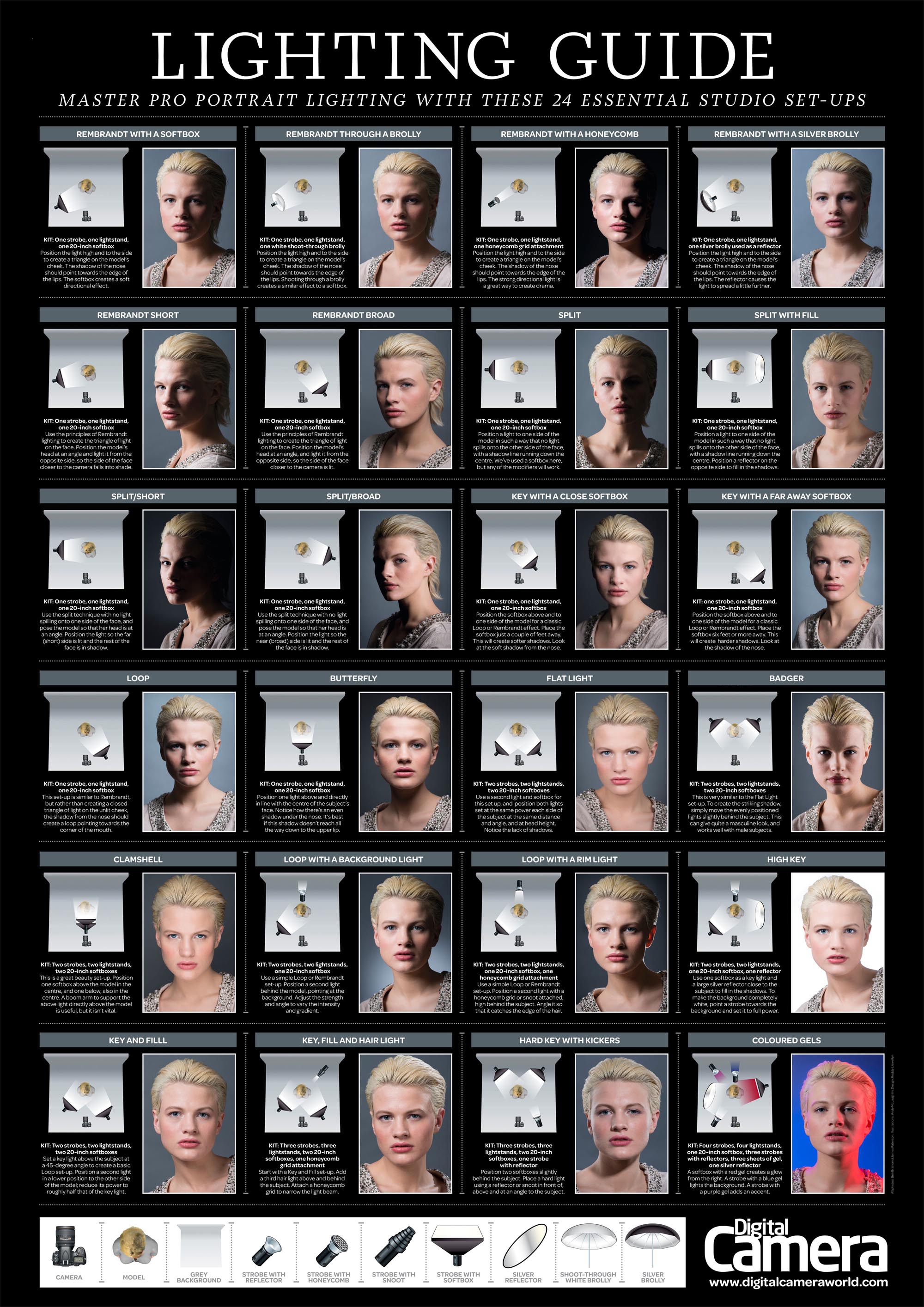
Composition – These are the basic lighting techniques you need to know for photography and film
Read more: Composition – These are the basic lighting techniques you need to know for photography and film
http://www.diyphotography.net/basic-lighting-techniques-need-know-photography-film/
Amongst the basic techniques, there’s…
1- Side lighting – Literally how it sounds, lighting a subject from the side when they’re faced toward you
2- Rembrandt lighting – Here the light is at around 45 degrees over from the front of the subject, raised and pointing down at 45 degrees
3- Back lighting – Again, how it sounds, lighting a subject from behind. This can help to add drama with silouettes
4- Rim lighting – This produces a light glowing outline around your subject
5- Key light – The main light source, and it’s not necessarily always the brightest light source
6- Fill light – This is used to fill in the shadows and provide detail that would otherwise be blackness
7- Cross lighting – Using two lights placed opposite from each other to light two subjects


COLLECTIONS
| Featured AI
| Design And Composition
| Explore posts
POPULAR SEARCHES
unreal | pipeline | virtual production | free | learn | photoshop | 360 | macro | google | nvidia | resolution | open source | hdri | real-time | photography basics | nuke
FEATURED POSTS
-
Godot Cheat Sheets
-
Emmanuel Tsekleves – Writing Research Papers
-
Yann Lecun: Meta AI, Open Source, Limits of LLMs, AGI & the Future of AI | Lex Fridman Podcast #416
-
Sensitivity of human eye
-
Types of Film Lights and their efficiency – CRI, Color Temperature and Luminous Efficacy
-
AI Search – Find The Best AI Tools & Apps
-
Google – Artificial Intelligence free courses
-
Python and TCL: Tips and Tricks for Foundry Nuke
Social Links
DISCLAIMER – Links and images on this website may be protected by the respective owners’ copyright. All data submitted by users through this site shall be treated as freely available to share.
