


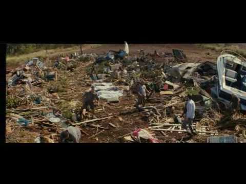
COMPOSITION


DESIGN
-
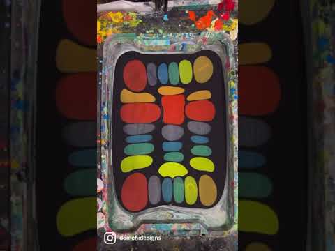
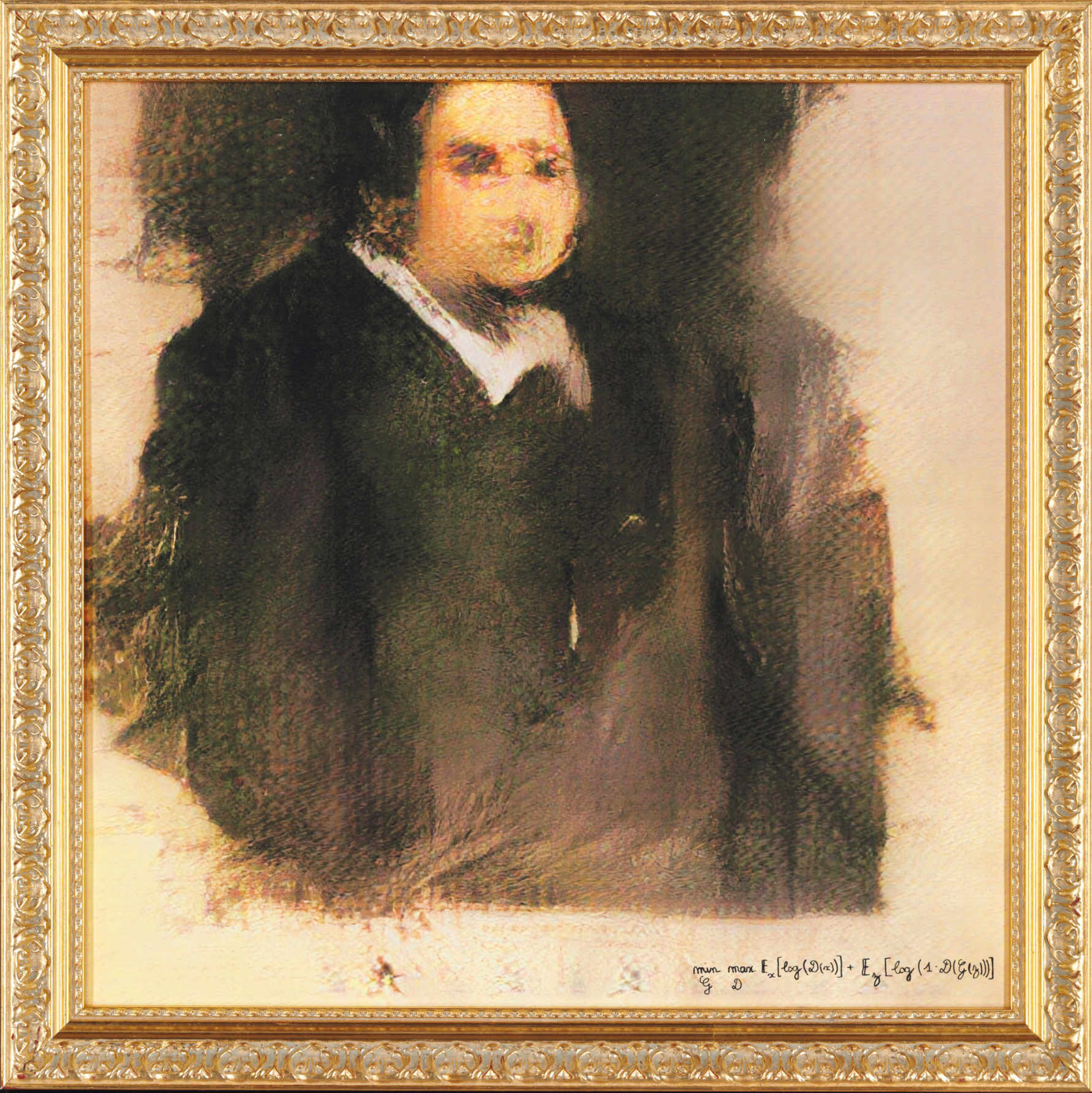
A.I. Algorithm art fetches US$432,500 at Christie auction
Read more: A.I. Algorithm art fetches US$432,500 at Christie auctionwww.ctvnews.ca/entertainment/algorithm-art-fetches-us-432-500-at-christie-s-auction-1.4150620
www.christies.com/features/A-collaboration-between-two-artists-one-human-one-a-machine-9332-1.aspx


COLOR
-
Björn Ottosson – OKlch color space
Read more: Björn Ottosson – OKlch color spaceBjörn Ottosson proposed OKlch in 2020 to create a color space that can closely mimic how color is perceived by the human eye, predicting perceived lightness, chroma, and hue.
The OK in OKLCH stands for Optimal Color.
- L: Lightness (the perceived brightness of the color)
- C: Chroma (the intensity or saturation of the color)
- H: Hue (the actual color, such as red, blue, green, etc.)

Also read:
-
Willem Zwarthoed – Aces gamut in VFX production pdf
Read more: Willem Zwarthoed – Aces gamut in VFX production pdfhttps://www.provideocoalition.com/color-management-part-12-introducing-aces/
Local copy:
https://www.slideshare.net/hpduiker/acescg-a-common-color-encoding-for-visual-effects-applications
-
Victor Perez – The Color Management Handbook for Visual Effects Artists
Read more: Victor Perez – The Color Management Handbook for Visual Effects ArtistsDigital Color Principles, Color Management Fundamentals & ACES Workflows

-
Capturing textures albedo
Read more: Capturing textures albedoBuilding a Portable PBR Texture Scanner by Stephane Lb
http://rtgfx.com/pbr-texture-scanner/

How To Split Specular And Diffuse In Real Images, by John Hable
http://filmicworlds.com/blog/how-to-split-specular-and-diffuse-in-real-images/Capturing albedo using a Spectralon
https://www.activision.com/cdn/research/Real_World_Measurements_for_Call_of_Duty_Advanced_Warfare.pdfReal_World_Measurements_for_Call_of_Duty_Advanced_Warfare.pdf
Spectralon is a teflon-based pressed powderthat comes closest to being a pure Lambertian diffuse material that reflects 100% of all light. If we take an HDR photograph of the Spectralon alongside the material to be measured, we can derive thediffuse albedo of that material.

The process to capture diffuse reflectance is very similar to the one outlined by Hable.
1. We put a linear polarizing filter in front of the camera lens and a second linear polarizing filterin front of a modeling light or a flash such that the two filters are oriented perpendicular to eachother, i.e. cross polarized.
2. We place Spectralon close to and parallel with the material we are capturing and take brack-eted shots of the setup7. Typically, we’ll take nine photographs, from -4EV to +4EV in 1EVincrements.
3. We convert the bracketed shots to a linear HDR image. We found that many HDR packagesdo not produce an HDR image in which the pixel values are linear. PTGui is an example of apackage which does generate a linear HDR image. At this point, because of the cross polarization,the image is one of surface diffuse response.
4. We open the file in Photoshop and normalize the image by color picking the Spectralon, filling anew layer with that color and setting that layer to “Divide”. This sets the Spectralon to 1 in theimage. All other color values are relative to this so we can consider them as diffuse albedo.


LIGHTING
-
Magnific.ai Relight – change the entire lighting of a scene
Read more: Magnific.ai Relight – change the entire lighting of a scene
It’s a new Magnific spell that allows you to change the entire lighting of a scene and, optionally, the background with just:
1/ A prompt OR
2/ A reference image OR
3/ A light map (drawing your own lights)https://x.com/javilopen/status/1805274155065176489


-
Photography basics: Exposure Value vs Photographic Exposure vs Il/Luminance vs Pixel luminance measurements
Read more: Photography basics: Exposure Value vs Photographic Exposure vs Il/Luminance vs Pixel luminance measurementsAlso see: https://www.pixelsham.com/2015/05/16/how-aperture-shutter-speed-and-iso-affect-your-photos/
In photography, exposure value (EV) is a number that represents a combination of a camera’s shutter speed and f-number, such that all combinations that yield the same exposure have the same EV (for any fixed scene luminance).
The EV concept was developed in an attempt to simplify choosing among combinations of equivalent camera settings. Although all camera settings with the same EV nominally give the same exposure, they do not necessarily give the same picture. EV is also used to indicate an interval on the photographic exposure scale. 1 EV corresponding to a standard power-of-2 exposure step, commonly referred to as a stop
EV 0 corresponds to an exposure time of 1 sec and a relative aperture of f/1.0. If the EV is known, it can be used to select combinations of exposure time and f-number.Note EV does not equal to photographic exposure. Photographic Exposure is defined as how much light hits the camera’s sensor. It depends on the camera settings mainly aperture and shutter speed. Exposure value (known as EV) is a number that represents the exposure setting of the camera.
Thus, strictly, EV is not a measure of luminance (indirect or reflected exposure) or illuminance (incidentl exposure); rather, an EV corresponds to a luminance (or illuminance) for which a camera with a given ISO speed would use the indicated EV to obtain the nominally correct exposure. Nonetheless, it is common practice among photographic equipment manufacturers to express luminance in EV for ISO 100 speed, as when specifying metering range or autofocus sensitivity.
The exposure depends on two things: how much light gets through the lenses to the camera’s sensor and for how long the sensor is exposed. The former is a function of the aperture value while the latter is a function of the shutter speed. Exposure value is a number that represents this potential amount of light that could hit the sensor. It is important to understand that exposure value is a measure of how exposed the sensor is to light and not a measure of how much light actually hits the sensor. The exposure value is independent of how lit the scene is. For example a pair of aperture value and shutter speed represents the same exposure value both if the camera is used during a very bright day or during a dark night.
Each exposure value number represents all the possible shutter and aperture settings that result in the same exposure. Although the exposure value is the same for different combinations of aperture values and shutter speeds the resulting photo can be very different (the aperture controls the depth of field while shutter speed controls how much motion is captured).
EV 0.0 is defined as the exposure when setting the aperture to f-number 1.0 and the shutter speed to 1 second. All other exposure values are relative to that number. Exposure values are on a base two logarithmic scale. This means that every single step of EV – plus or minus 1 – represents the exposure (actual light that hits the sensor) being halved or doubled.Formulas
(more…) -
HDRI shooting and editing by Xuan Prada and Greg Zaal
Read more: HDRI shooting and editing by Xuan Prada and Greg Zaalwww.xuanprada.com/blog/2014/11/3/hdri-shooting
http://blog.gregzaal.com/2016/03/16/make-your-own-hdri/
http://blog.hdrihaven.com/how-to-create-high-quality-hdri/
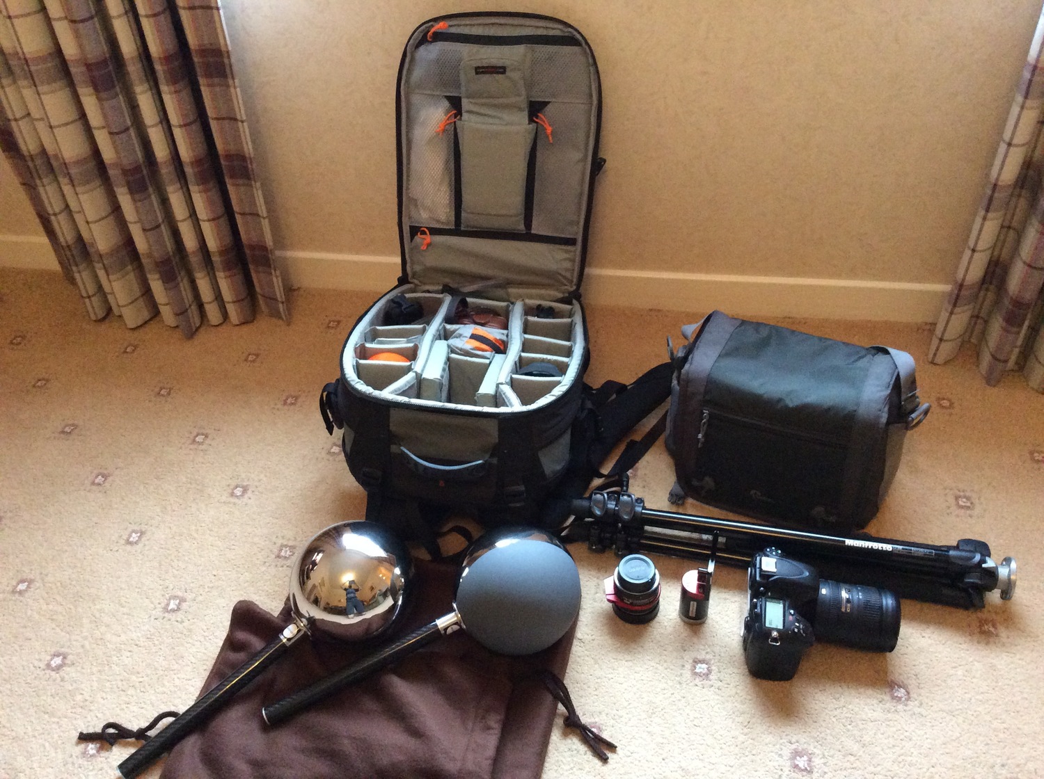
Shooting checklist
- Full coverage of the scene (fish-eye shots)
- Backplates for look-development (including ground or floor)
- Macbeth chart for white balance
- Grey ball for lighting calibration
- Chrome ball for lighting orientation
- Basic scene measurements
- Material samples
- Individual HDR artificial lighting sources if required
Methodology
(more…)


COLLECTIONS
| Featured AI
| Design And Composition
| Explore posts
POPULAR SEARCHES
unreal | pipeline | virtual production | free | learn | photoshop | 360 | macro | google | nvidia | resolution | open source | hdri | real-time | photography basics | nuke
FEATURED POSTS
-
Canva bought Affinity – Now Affinity Photo and Affinity Designer are… GONE?!
-
Glossary of Lighting Terms – cheat sheet
-
Most common ways to smooth 3D prints
-
Game Development tips
-
Cinematographers Blueprint 300dpi poster
-
Types of AI Explained in a few Minutes – AI Glossary
-
Decart AI Mirage – The first ever World Transformation Model – turning any video, game, or camera feed into a new digital world, in real time
-
Photography basics: Lumens vs Candelas (candle) vs Lux vs FootCandle vs Watts vs Irradiance vs Illuminance
Social Links
DISCLAIMER – Links and images on this website may be protected by the respective owners’ copyright. All data submitted by users through this site shall be treated as freely available to share.
