


COMPOSITION
-
SlowMoVideo – How to make a slow motion shot with the open source program
Read more: SlowMoVideo – How to make a slow motion shot with the open source programhttp://slowmovideo.granjow.net/
slowmoVideo is an OpenSource program that creates slow-motion videos from your footage.
Slow motion cinematography is the result of playing back frames for a longer duration than they were exposed. For example, if you expose 240 frames of film in one second, then play them back at 24 fps, the resulting movie is 10 times longer (slower) than the original filmed event….
Film cameras are relatively simple mechanical devices that allow you to crank up the speed to whatever rate the shutter and pull-down mechanism allow. Some film cameras can operate at 2,500 fps or higher (although film shot in these cameras often needs some readjustment in postproduction). Video, on the other hand, is always captured, recorded, and played back at a fixed rate, with a current limit around 60fps. This makes extreme slow motion effects harder to achieve (and less elegant) on video, because slowing down the video results in each frame held still on the screen for a long time, whereas with high-frame-rate film there are plenty of frames to fill the longer durations of time. On video, the slow motion effect is more like a slide show than smooth, continuous motion.
One obvious solution is to shoot film at high speed, then transfer it to video (a case where film still has a clear advantage, sorry George). Another possibility is to cross dissolve or blur from one frame to the next. This adds a smooth transition from one still frame to the next. The blur reduces the sharpness of the image, and compared to slowing down images shot at a high frame rate, this is somewhat of a cheat. However, there isn’t much you can do about it until video can be recorded at much higher rates. Of course, many film cameras can’t shoot at high frame rates either, so the whole super-slow-motion endeavor is somewhat specialized no matter what medium you are using. (There are some high speed digital cameras available now that allow you to capture lots of digital frames directly to your computer, so technology is starting to catch up with film. However, this feature isn’t going to appear in consumer camcorders any time soon.)


DESIGN
COLOR
-
What Is The Resolution and view coverage Of The human Eye. And what distance is TV at best?
Read more: What Is The Resolution and view coverage Of The human Eye. And what distance is TV at best?
https://www.discovery.com/science/mexapixels-in-human-eye
About 576 megapixels for the entire field of view.
Consider a view in front of you that is 90 degrees by 90 degrees, like looking through an open window at a scene. The number of pixels would be:
90 degrees * 60 arc-minutes/degree * 1/0.3 * 90 * 60 * 1/0.3 = 324,000,000 pixels (324 megapixels).At any one moment, you actually do not perceive that many pixels, but your eye moves around the scene to see all the detail you want. But the human eye really sees a larger field of view, close to 180 degrees. Let’s be conservative and use 120 degrees for the field of view. Then we would see:
120 * 120 * 60 * 60 / (0.3 * 0.3) = 576 megapixels.
Or.
7 megapixels for the 2 degree focus arc… + 1 megapixel for the rest.
https://clarkvision.com/articles/eye-resolution.html
Details in the post
-
Björn Ottosson – OKHSV and OKHSL – Two new color spaces for color picking
Read more: Björn Ottosson – OKHSV and OKHSL – Two new color spaces for color pickinghttps://bottosson.github.io/misc/colorpicker
https://bottosson.github.io/posts/colorpicker/
https://www.smashingmagazine.com/2024/10/interview-bjorn-ottosson-creator-oklab-color-space/
One problem with sRGB is that in a gradient between blue and white, it becomes a bit purple in the middle of the transition. That’s because sRGB really isn’t created to mimic how the eye sees colors; rather, it is based on how CRT monitors work. That means it works with certain frequencies of red, green, and blue, and also the non-linear coding called gamma. It’s a miracle it works as well as it does, but it’s not connected to color perception. When using those tools, you sometimes get surprising results, like purple in the gradient.

There were also attempts to create simple models matching human perception based on XYZ, but as it turned out, it’s not possible to model all color vision that way. Perception of color is incredibly complex and depends, among other things, on whether it is dark or light in the room and the background color it is against. When you look at a photograph, it also depends on what you think the color of the light source is. The dress is a typical example of color vision being very context-dependent. It is almost impossible to model this perfectly.
I based Oklab on two other color spaces, CIECAM16 and IPT. I used the lightness and saturation prediction from CIECAM16, which is a color appearance model, as a target. I actually wanted to use the datasets used to create CIECAM16, but I couldn’t find them.
IPT was designed to have better hue uniformity. In experiments, they asked people to match light and dark colors, saturated and unsaturated colors, which resulted in a dataset for which colors, subjectively, have the same hue. IPT has a few other issues but is the basis for hue in Oklab.
In the Munsell color system, colors are described with three parameters, designed to match the perceived appearance of colors: Hue, Chroma and Value. The parameters are designed to be independent and each have a uniform scale. This results in a color solid with an irregular shape. The parameters are designed to be independent and each have a uniform scale. This results in a color solid with an irregular shape. Modern color spaces and models, such as CIELAB, Cam16 and Björn Ottosson own Oklab, are very similar in their construction.

By far the most used color spaces today for color picking are HSL and HSV, two representations introduced in the classic 1978 paper “Color Spaces for Computer Graphics”. HSL and HSV designed to roughly correlate with perceptual color properties while being very simple and cheap to compute.
Today HSL and HSV are most commonly used together with the sRGB color space.

One of the main advantages of HSL and HSV over the different Lab color spaces is that they map the sRGB gamut to a cylinder. This makes them easy to use since all parameters can be changed independently, without the risk of creating colors outside of the target gamut.

The main drawback on the other hand is that their properties don’t match human perception particularly well.
Reconciling these conflicting goals perfectly isn’t possible, but given that HSV and HSL don’t use anything derived from experiments relating to human perception, creating something that makes a better tradeoff does not seem unreasonable.
With this new lightness estimate, we are ready to look into the construction of Okhsv and Okhsl.


-
OpenColorIO standard
Read more: OpenColorIO standardhttps://www.provideocoalition.com/color-management-part-11-introducing-opencolorio/
OpenColorIO (OCIO) is a new open source project from Sony Imageworks.
Based on development started in 2003, OCIO enables color transforms and image display to be handled in a consistent manner across multiple graphics applications. Unlike other color management solutions, OCIO is geared towards motion-picture post production, with an emphasis on visual effects and animation color pipelines.

-
Tim Kang – calibrated white light values in sRGB color space
Read more: Tim Kang – calibrated white light values in sRGB color space8bit sRGB encoded
2000K 255 139 22
2700K 255 172 89
3000K 255 184 109
3200K 255 190 122
4000K 255 211 165
4300K 255 219 178
D50 255 235 205
D55 255 243 224
D5600 255 244 227
D6000 255 249 240
D65 255 255 255
D10000 202 221 255
D20000 166 196 2558bit Rec709 Gamma 2.4
2000K 255 145 34
2700K 255 177 97
3000K 255 187 117
3200K 255 193 129
4000K 255 214 170
4300K 255 221 182
D50 255 236 208
D55 255 243 226
D5600 255 245 229
D6000 255 250 241
D65 255 255 255
D10000 204 222 255
D20000 170 199 2558bit Display P3 encoded
2000K 255 154 63
2700K 255 185 109
3000K 255 195 127
3200K 255 201 138
4000K 255 219 176
4300K 255 225 187
D50 255 239 212
D55 255 245 228
D5600 255 246 231
D6000 255 251 242
D65 255 255 255
D10000 208 223 255
D20000 175 199 25510bit Rec2020 PQ (100 nits)
2000K 520 435 273
2700K 520 466 358
3000K 520 475 384
3200K 520 480 399
4000K 520 495 446
4300K 520 500 458
D50 520 510 482
D55 520 514 497
D5600 520 514 500
D6000 520 517 509
D65 520 520 520
D10000 479 489 520
D20000 448 464 520
-
RawTherapee – a free, open source, cross-platform raw image and HDRi processing program
Read more: RawTherapee – a free, open source, cross-platform raw image and HDRi processing program5.10 of this tool includes excellent tools to clean up cr2 and cr3 used on set to support HDRI processing.
Converting raw to AcesCG 32 bit tiffs with metadata.


-
Virtual Production volumes study
Read more: Virtual Production volumes studyColor Fidelity in LED Volumes
https://theasc.com/articles/color-fidelity-in-led-volumes
Virtual Production Glossary
https://vpglossary.com/What is Virtual Production – In depth analysis
https://www.leadingledtech.com/what-is-a-led-virtual-production-studio-in-depth-technical-analysis/
A comparison of LED panels for use in Virtual Production:
Findings and recommendations
https://eprints.bournemouth.ac.uk/36826/1/LED_Comparison_White_Paper%281%29.pdf


![[gamma correction test]](http://www.madore.org/~david/misc/color/gammatest.png "sRGB gamma correction test")

LIGHTING
-
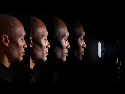
Composition and The Expressive Nature Of Light
Read more: Composition and The Expressive Nature Of Lighthttp://www.huffingtonpost.com/bill-danskin/post_12457_b_10777222.html
George Sand once said “ The artist vocation is to send light into the human heart.”

-
Simulon – a Hollywood production studio app in the hands of an independent creator with access to consumer hardware, LDRi to HDRi through ML
Read more: Simulon – a Hollywood production studio app in the hands of an independent creator with access to consumer hardware, LDRi to HDRi through MLDivesh Naidoo: The video below was made with a live in-camera preview and auto-exposure matching, no camera solve, no HDRI capture and no manual compositing setup. Using the new Simulon phone app.
LDR to HDR through ML
https://simulon.typeform.com/betatest
(more…)Process example
-
Polarised vs unpolarized filtering
Read more: Polarised vs unpolarized filteringA light wave that is vibrating in more than one plane is referred to as unpolarized light. …
Polarized light waves are light waves in which the vibrations occur in a single plane. The process of transforming unpolarized light into polarized light is known as polarization.

en.wikipedia.org/wiki/Polarizing_filter_(photography)
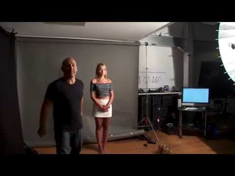
The most common use of polarized technology is to reduce lighting complexity on the subject.
(more…)
Details such as glare and hard edges are not removed, but greatly reduced. -
Convert between light exposure and intensity
Read more: Convert between light exposure and intensityimport math,sys def Exposure2Intensity(exposure): exp = float(exposure) result = math.pow(2,exp) print(result) Exposure2Intensity(0) def Intensity2Exposure(intensity): inarg = float(intensity) if inarg == 0: print("Exposure of zero intensity is undefined.") return if inarg < 1e-323: inarg = max(inarg, 1e-323) print("Exposure of negative intensities is undefined. Clamping to a very small value instead (1e-323)") result = math.log(inarg, 2) print(result) Intensity2Exposure(0.1)Why Exposure?
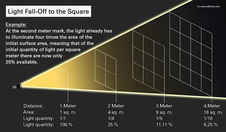
Exposure is a stop value that multiplies the intensity by 2 to the power of the stop. Increasing exposure by 1 results in double the amount of light.
Artists think in “stops.” Doubling or halving brightness is easy math and common in grading and look-dev.
Exposure counts doublings in whole stops:- +1 stop = ×2 brightness
- −1 stop = ×0.5 brightness
This gives perceptually even controls across both bright and dark values.
Why Intensity?
Intensity is linear.
It’s what render engines and compositors expect when:- Summing values
- Averaging pixels
- Multiplying or filtering pixel data
Use intensity when you need the actual math on pixel/light data.
Formulas (from your Python)
- Intensity from exposure: intensity = 2**exposure
- Exposure from intensity: exposure = log₂(intensity)
Guardrails:
- Intensity must be > 0 to compute exposure.
- If intensity = 0 → exposure is undefined.
- Clamp tiny values (e.g.
1e−323) before using log₂.
Use Exposure (stops) when…
- You want artist-friendly sliders (−5…+5 stops)
- Adjusting look-dev or grading in even stops
- Matching plates with quick ±1 stop tweaks
- Tweening brightness changes smoothly across ranges
Use Intensity (linear) when…
- Storing raw pixel/light values
- Multiplying textures or lights by a gain
- Performing sums, averages, and filters
- Feeding values to render engines expecting linear data
Examples
- +2 stops → 2**2 = 4.0 (×4)
- +1 stop → 2**1 = 2.0 (×2)
- 0 stop → 2**0 = 1.0 (×1)
- −1 stop → 2**(−1) = 0.5 (×0.5)
- −2 stops → 2**(−2) = 0.25 (×0.25)
- Intensity 0.1 → exposure = log₂(0.1) ≈ −3.32
Rule of thumb
Think in stops (exposure) for controls and matching.
Compute in linear (intensity) for rendering and math. -
What is the Light Field?
Read more: What is the Light Field?http://lightfield-forum.com/what-is-the-lightfield/
The light field consists of the total of all light rays in 3D space, flowing through every point and in every direction.
How to Record a Light Field
- a single, robotically controlled camera
- a rotating arc of cameras
- an array of cameras or camera modules
- a single camera or camera lens fitted with a microlens array


-
Narcis Calin’s Galaxy Engine – A free, open source simulation software
Read more: Narcis Calin’s Galaxy Engine – A free, open source simulation softwareThis 2025 I decided to start learning how to code, so I installed Visual Studio and I started looking into C++. After days of watching tutorials and guides about the basics of C++ and programming, I decided to make something physics-related. I started with a dot that fell to the ground and then I wanted to simulate gravitational attraction, so I made 2 circles attracting each other. I thought it was really cool to see something I made with code actually work, so I kept building on top of that small, basic program. And here we are after roughly 8 months of learning programming. This is Galaxy Engine, and it is a simulation software I have been making ever since I started my learning journey. It currently can simulate gravity, dark matter, galaxies, the Big Bang, temperature, fluid dynamics, breakable solids, planetary interactions, etc. The program can run many tens of thousands of particles in real time on the CPU thanks to the Barnes-Hut algorithm, mixed with Morton curves. It also includes its own PBR 2D path tracer with BVH optimizations. The path tracer can simulate a bunch of stuff like diffuse lighting, specular reflections, refraction, internal reflection, fresnel, emission, dispersion, roughness, IOR, nested IOR and more! I tried to make the path tracer closer to traditional 3D render engines like V-Ray. I honestly never imagined I would go this far with programming, and it has been an amazing learning experience so far. I think that mixing this knowledge with my 3D knowledge can unlock countless new possibilities. In case you are curious about Galaxy Engine, I made it completely free and Open-Source so that anyone can build and compile it locally! You can find the source code in GitHub
https://github.com/NarcisCalin/Galaxy-Engine
-
Light properties
Read more: Light propertiesHow It Works – Issue 114
https://www.howitworksdaily.com/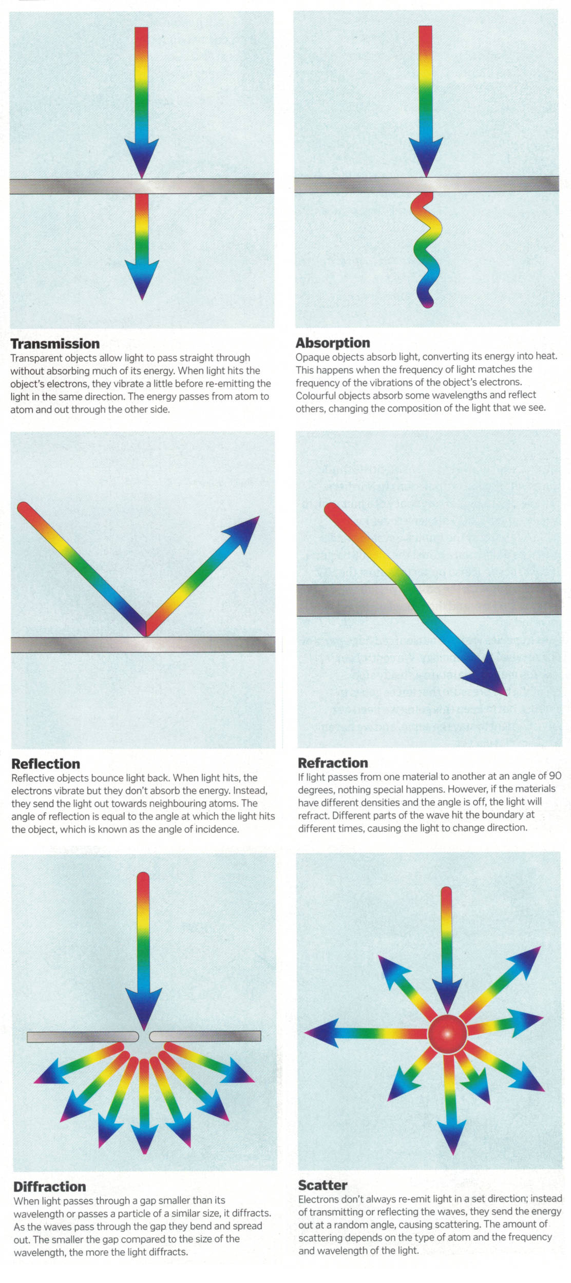


COLLECTIONS
| Featured AI
| Design And Composition
| Explore posts
POPULAR SEARCHES
unreal | pipeline | virtual production | free | learn | photoshop | 360 | macro | google | nvidia | resolution | open source | hdri | real-time | photography basics | nuke
FEATURED POSTS
-
Web vs Printing or digital RGB vs CMYK
-
JavaScript how-to free resources
-
Types of AI Explained in a few Minutes – AI Glossary
-
Photography basics: How Exposure Stops (Aperture, Shutter Speed, and ISO) Affect Your Photos – cheat sheet cards
-
Daniele Tosti Interview for the magazine InCG, Taiwan, Issue 28, 201609
-
AI and the Law – Netflix : Using Generative AI in Content Production
-
MiniMax-Remover – Taming Bad Noise Helps Video Object Removal Rotoscoping
-
SourceTree vs Github Desktop – Which one to use
Social Links
DISCLAIMER – Links and images on this website may be protected by the respective owners’ copyright. All data submitted by users through this site shall be treated as freely available to share.
