Spectral sensitivity of eye is influenced by light intensity. And the light intensity determines the level of activity of cones cell and rod cell. This is the main characteristic of human vision. Sensitivity to individual colors, in other words, wavelengths of the light spectrum, is explained by the RGB (red-green-blue) theory. This theory assumed that there are three kinds of cones. It’s selectively sensitive to red (700-630 nm), green (560-500 nm), and blue (490-450 nm) light. And their mutual interaction allow to perceive all colors of the spectrum.
One problem with sRGB is that in a gradient between blue and white, it becomes a bit purple in the middle of the transition. That’s because sRGB really isn’t created to mimic how the eye sees colors; rather, it is based on how CRT monitors work. That means it works with certain frequencies of red, green, and blue, and also the non-linear coding called gamma. It’s a miracle it works as well as it does, but it’s not connected to color perception. When using those tools, you sometimes get surprising results, like purple in the gradient.
There were also attempts to create simple models matching human perception based on XYZ, but as it turned out, it’s not possible to model all color vision that way. Perception of color is incredibly complex and depends, among other things, on whether it is dark or light in the room and the background color it is against. When you look at a photograph, it also depends on what you think the color of the light source is. The dress is a typical example of color vision being very context-dependent. It is almost impossible to model this perfectly.
I based Oklab on two other color spaces, CIECAM16 and IPT. I used the lightness and saturation prediction from CIECAM16, which is a color appearance model, as a target. I actually wanted to use the datasets used to create CIECAM16, but I couldn’t find them.
IPT was designed to have better hue uniformity. In experiments, they asked people to match light and dark colors, saturated and unsaturated colors, which resulted in a dataset for which colors, subjectively, have the same hue. IPT has a few other issues but is the basis for hue in Oklab.
In the Munsell color system, colors are described with three parameters, designed to match the perceived appearance of colors: Hue, Chroma and Value. The parameters are designed to be independent and each have a uniform scale. This results in a color solid with an irregular shape. The parameters are designed to be independent and each have a uniform scale. This results in a color solid with an irregular shape. Modern color spaces and models, such as CIELAB, Cam16 and Björn Ottosson own Oklab, are very similar in their construction.
By far the most used color spaces today for color picking are HSL and HSV, two representations introduced in the classic 1978 paper “Color Spaces for Computer Graphics”. HSL and HSV designed to roughly correlate with perceptual color properties while being very simple and cheap to compute.
Today HSL and HSV are most commonly used together with the sRGB color space.
One of the main advantages of HSL and HSV over the different Lab color spaces is that they map the sRGB gamut to a cylinder. This makes them easy to use since all parameters can be changed independently, without the risk of creating colors outside of the target gamut.
The main drawback on the other hand is that their properties don’t match human perception particularly well.
Reconciling these conflicting goals perfectly isn’t possible, but given that HSV and HSL don’t use anything derived from experiments relating to human perception, creating something that makes a better tradeoff does not seem unreasonable.
With this new lightness estimate, we are ready to look into the construction of Okhsv and Okhsl.
Colour is an open-source Python package providing a comprehensive number of algorithms and datasets for colour science. It is freely available under the BSD-3-Clause terms.
The 2011 Best Illusion of the Year uses motion to render color changes invisible, and so reveals a quirk in our visual systems that is new to scientists.
“It is a really beautiful effect, revealing something about how our visual system works that we didn’t know before,” said Daniel Simons, a professor at the University of Illinois, Champaign-Urbana. Simons studies visual cognition, and did not work on this illusion. Before its creation, scientists didn’t know that motion had this effect on perception, Simons said.
A viewer stares at a speck at the center of a ring of colored dots, which continuously change color. When the ring begins to rotate around the speck, the color changes appear to stop. But this is an illusion. For some reason, the motion causes our visual system to ignore the color changes. (You can, however, see the color changes if you follow the rotating circles with your eyes.)
Most software around us today are decent at accurately displaying colors. Processing of colors is another story unfortunately, and is often done badly.
To understand what the problem is, let’s start with an example of three ways of blending green and magenta:
Perceptual blend – A smooth transition using a model designed to mimic human perception of color. The blending is done so that the perceived brightness and color varies smoothly and evenly.
Linear blend – A model for blending color based on how light behaves physically. This type of blending can occur in many ways naturally, for example when colors are blended together by focus blur in a camera or when viewing a pattern of two colors at a distance.
sRGB blend – This is how colors would normally be blended in computer software, using sRGB to represent the colors.
Let’s look at some more examples of blending of colors, to see how these problems surface more practically. The examples use strong colors since then the differences are more pronounced. This is using the same three ways of blending colors as the first example.
Instead of making it as easy as possible to work with color, most software make it unnecessarily hard, by doing image processing with representations not designed for it. Approximating the physical behavior of light with linear RGB models is one easy thing to do, but more work is needed to create image representations tailored for image processing and human perception.
Display Referred it is tied to the target hardware, as such it bakes color requirements into every type of media output request.
Scene Referred uses a common unified wide gamut and targeting audience through CDL and DI libraries instead.
So that color information stays untouched and only “transformed” as/when needed.
Sources:
– Victor Perez – Color Management Fundamentals & ACES Workflows in Nuke
– https://z-fx.nl/ColorspACES.pdf – Wicus
The Manuka rendering architecture has been designed in the spirit of the classic reyes rendering architecture. In its core, reyes is based on stochastic rasterisation of micropolygons, facilitating depth of field, motion blur, high geometric complexity,and programmable shading.
This is commonly achieved with Monte Carlo path tracing, using a paradigm often called shade-on-hit, in which the renderer alternates tracing rays with running shaders on the various ray hits. The shaders take the role of generating the inputs of the local material structure which is then used bypath sampling logic to evaluate contributions and to inform what further rays to cast through the scene.
Over the years, however, the expectations have risen substantially when it comes to image quality. Computing pictures which are indistinguishable from real footage requires accurate simulation of light transport, which is most often performed using some variant of Monte Carlo path tracing. Unfortunately this paradigm requires random memory accesses to the whole scene and does not lend itself well to a rasterisation approach at all.
Manuka is both a uni-directional and bidirectional path tracer and encompasses multiple importance sampling (MIS). Interestingly, and importantly for production character skin work, it is the first major production renderer to incorporate spectral MIS in the form of a new ‘Hero Spectral Sampling’ technique, which was recently published at Eurographics Symposium on Rendering 2014.
Manuka propose a shade-before-hit paradigm in-stead and minimise I/O strain (and some memory costs) on the system, leveraging locality of reference by running pattern generation shaders before we execute light transport simulation by path sampling, “compressing” any bvh structure as needed, and as such also limiting duplication of source data.
The difference with reyes is that instead of baking colors into the geometry like in Reyes, manuka bakes surface closures. This means that light transport is still calculated with path tracing, but all texture lookups etc. are done up-front and baked into the geometry.
The main drawback with this method is that geometry has to be tessellated to its highest, stable topology before shading can be evaluated properly. As such, the high cost to first pixel. Even a basic 4 vertices square becomes a much more complex model with this approach.
Manuka use the RenderMan Shading Language (rsl) for programmable shading [Pixar Animation Studios 2015], but we do not invoke rsl shaders when intersecting a ray with a surface (often called shade-on-hit). Instead, we pre-tessellate and pre-shade all the input geometry in the front end of the renderer.
This way, we can efficiently order shading computations to sup-port near-optimal texture locality, vectorisation, and parallelism. This system avoids repeated evaluation of shaders at the same surface point, and presents a minimal amount of memory to be accessed during light transport time. An added benefit is that the acceleration structure for ray tracing (abounding volume hierarchy, bvh) is built once on the final tessellated geometry, which allows us to ray trace more efficiently than multi-level bvhs and avoids costly caching of on-demand tessellated micropolygons and the associated scheduling issues.
For the shading reasons above, in terms of AOVs, the studio approach is to succeed at combining complex shading with ray paths in the render rather than pass a multi-pass render to compositing.
For the Spectral Rendering component. The light transport stage is fully spectral, using a continuously sampled wavelength which is traced with each path and used to apply the spectral camera sensitivity of the sensor. This allows for faithfully support any degree of observer metamerism as the camera footage they are intended to match as well as complex materials which require wavelength dependent phenomena such as diffraction, dispersion, interference, iridescence, or chromatic extinction and Rayleigh scattering in participating media.
As opposed to the original reyes paper, we use bilinear interpolation of these bsdf inputs later when evaluating bsdfs per pathv ertex during light transport4. This improves temporal stability of geometry which moves very slowly with respect to the pixel raster
In terms of the pipeline, everything rendered at Weta was already completely interwoven with their deep data pipeline. Manuka very much was written with deep data in mind. Here, Manuka not so much extends the deep capabilities, rather it fully matches the already extremely complex and powerful setup Weta Digital already enjoy with RenderMan. For example, an ape in a scene can be selected, its ID is available and a NUKE artist can then paint in 3D say a hand and part of the way up the neutral posed ape.
We called our system Manuka, as a respectful nod to reyes: we had heard a story froma former ILM employee about how reyes got its name from how fond the early Pixar people were of their lunches at Point Reyes, and decided to name our system after our surrounding natural environment, too. Manuka is a kind of tea tree very common in New Zealand which has very many very small leaves, in analogy to micropolygons ina tree structure for ray tracing. It also happens to be the case that Weta Digital’s main site is on Manuka Street.
sRGB: A standard “web”/computer-display RGB color space defined by IEC 61966-2-1. It’s used for most monitors, cameras, printers, and the vast majority of images on the Internet.
Rec. 709: An HD-video color space defined by ITU-R BT.709. It’s the go-to standard for HDTV broadcasts, Blu-ray discs, and professional video pipelines.
Why they exist
sRGB: Ensures consistent colors across different consumer devices (PCs, phones, webcams).
Rec. 709: Ensures consistent colors across video production and playback chains (cameras → editing → broadcast → TV).
What you’ll see
On your desktop or phone, images tagged sRGB will look “right” without extra tweaking.
On an HDTV or video-editing timeline, footage tagged Rec. 709 will display accurate contrast and hue on broadcast-grade monitors.
The cone angle of the sun refers to the angular diameter of the sun as observed from Earth, which is related to the apparent size of the sun in the sky.
The angular diameter of the sun, or the cone angle of the sunlight as perceived from Earth, is approximately 0.53 degrees on average. This value can vary slightly due to the elliptical nature of Earth’s orbit around the sun, but it generally stays within a narrow range.
Here’s a more precise breakdown:
Average Angular Diameter: About 0.53 degrees (31 arcminutes)
Minimum Angular Diameter: Approximately 0.52 degrees (when Earth is at aphelion, the farthest point from the sun)
Maximum Angular Diameter: Approximately 0.54 degrees (when Earth is at perihelion, the closest point to the sun)
This angular diameter remains relatively constant throughout the day because the sun’s distance from Earth does not change significantly over a single day.
To summarize, the cone angle of the sun’s light, or its angular diameter, is typically around 0.53 degrees, regardless of the time of day.
1 to 100% Stepless Dimming, 1500 Lux Brightness at 3.3′
LCD Info Screen. Powered by an L-series battery, D-Tap, or USB-C
Because the light has a variable color range of 3200 to 9500K, when the light is set to 5500K (daylight balanced) both sets of LEDs are on at full, providing the maximum brightness from this fixture when compared to using the light at 3200 or 9500K.
The LCD screen provides information on the fixture’s output as well as the charge state of the battery. The screen also indicates whether the adjustment knob is controlling brightness or color temperature. To switch from brightness to CCT or CCT to brightness, just apply a short press to the adjustment knob.
The included cold shoe ball joint adapter enables mounting the light to your camera’s accessory shoe via the 1/4″-20 threaded hole on the fixture. In addition, the bottom of the cold shoe foot features a 3/8″-16 threaded hole, and includes a 3/8″-16 to 1/4″-20 reducing bushing.
import math,sys

def Exposure2Intensity(exposure):
    exp = float(exposure)
    result = math.pow(2,exp)
    print(result)

Exposure2Intensity(0)

def Intensity2Exposure(intensity):
    inarg = float(intensity)

    if inarg == 0:
        print("Exposure of zero intensity is undefined.")
        return

    if inarg < 1e-323:
        inarg = max(inarg, 1e-323)
        print("Exposure of negative intensities is undefined. Clamping to a very small value instead (1e-323)")

    result = math.log(inarg, 2)
    print(result)

Intensity2Exposure(0.1)
Why Exposure?
Exposure is a stop value that multiplies the intensity by 2 to the power of the stop. Increasing exposure by 1 results in double the amount of light.
Artists think in “stops.” Doubling or halving brightness is easy math and common in grading and look-dev. Exposure counts doublings in whole stops:
+1 stop = ×2 brightness
−1 stop = ×0.5 brightness
This gives perceptually even controls across both bright and dark values.
Why Intensity?
Intensity is linear. It’s what render engines and compositors expect when:
Summing values
Averaging pixels
Multiplying or filtering pixel data
Use intensity when you need the actual math on pixel/light data.
Formulas (from your Python)
Intensity from exposure: intensity = 2**exposure
Exposure from intensity: exposure = log₂(intensity)
Guardrails:
Intensity must be > 0 to compute exposure.
If intensity = 0 → exposure is undefined.
Clamp tiny values (e.g. 1e−323) before using log₂.
Use Exposure (stops) when…
You want artist-friendly sliders (−5…+5 stops)
Adjusting look-dev or grading in even stops
Matching plates with quick ±1 stop tweaks
Tweening brightness changes smoothly across ranges
Use Intensity (linear) when…
Storing raw pixel/light values
Multiplying textures or lights by a gain
Performing sums, averages, and filters
Feeding values to render engines expecting linear data
Examples
+2 stops → 2**2 = 4.0 (×4)
+1 stop → 2**1 = 2.0 (×2)
0 stop → 2**0 = 1.0 (×1)
−1 stop → 2**(−1) = 0.5 (×0.5)
−2 stops → 2**(−2) = 0.25 (×0.25)
Intensity 0.1 → exposure = log₂(0.1) ≈ −3.32
Rule of thumb
Think in stops (exposure) for controls and matching. Compute in linear (intensity) for rendering and math.
DISCLAIMER – Links and images on this website may be protected by the respective owners’ copyright. All data submitted by users through this site shall be treated as freely available to share.


