Spectral sensitivity of eye is influenced by light intensity. And the light intensity determines the level of activity of cones cell and rod cell. This is the main characteristic of human vision. Sensitivity to individual colors, in other words, wavelengths of the light spectrum, is explained by the RGB (red-green-blue) theory. This theory assumed that there are three kinds of cones. It’s selectively sensitive to red (700-630 nm), green (560-500 nm), and blue (490-450 nm) light. And their mutual interaction allow to perceive all colors of the spectrum.
Display Referred it is tied to the target hardware, as such it bakes color requirements into every type of media output request.
Scene Referred uses a common unified wide gamut and targeting audience through CDL and DI libraries instead.
So that color information stays untouched and only “transformed” as/when needed.
Sources:
– Victor Perez – Color Management Fundamentals & ACES Workflows in Nuke
– https://z-fx.nl/ColorspACES.pdf – Wicus
Artificial light sources, not unlike the diverse phases of natural light, vary considerably in their properties. As a result, some lamps render an object’s color better than others do.
The most important criterion for assessing the color-rendering ability of any lamp is its spectral power distribution curve.
Natural daylight varies too much in strength and spectral composition to be taken seriously as a lighting standard for grading and dealing colored stones. For anything to be a standard, it must be constant in its properties, which natural light is not.
For dealers in particular to make the transition from natural light to an artificial light source, that source must offer:
1- A degree of illuminance at least as strong as the common phases of natural daylight.
2- Spectral properties identical or comparable to a phase of natural daylight.
A source combining these two things makes gems appear much the same as when viewed under a given phase of natural light. From the viewpoint of many dealers, this corresponds to a naturalappearance.
The 6000° Kelvin xenon short-arc lamp appears closest to meeting the criteria for a standard light source. Besides the strong illuminance this lamp affords, its spectrum is very similar to CIE standard illuminants of similar color temperature.
Answering the question that is often asked, “Do I need to use ACEScg to display an sRGB monitor in the end?” (Demonstration shown at an in-house seminar) Comparison of scanlineRender output with extreme color lights on color charts with sRGB/ACREScg in color – OCIO -working space in Nuke
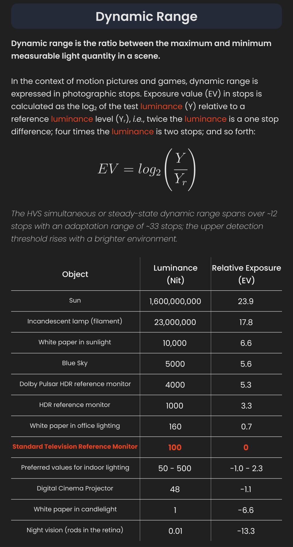
In photography, exposure value (EV) is a number that represents a combination of a camera’s shutter speed and f-number, such that all combinations that yield the same exposure have the same EV (for any fixed scene luminance).
The EV concept was developed in an attempt to simplify choosing among combinations of equivalent camera settings. Although all camera settings with the same EV nominally give the same exposure, they do not necessarily give the same picture. EV is also used to indicate an interval on the photographic exposure scale. 1 EV corresponding to a standard power-of-2 exposure step, commonly referred to as a stop
EV 0 corresponds to an exposure time of 1 sec and a relative aperture of f/1.0. If the EV is known, it can be used to select combinations of exposure time and f-number.
Note EV does not equal to photographic exposure. Photographic Exposureis defined as how much light hits the camera’s sensor. It depends on the camera settings mainly aperture and shutter speed. Exposure value (known as EV) is a number that represents theexposure setting of the camera.
Thus, strictly, EV is not a measure of luminance (indirect or reflected exposure) or illuminance (incidentl exposure); rather, an EV corresponds to a luminance (or illuminance) for which a camera with a given ISO speed would use the indicated EV to obtain the nominally correct exposure. Nonetheless, it is common practice among photographic equipment manufacturers to express luminance in EV for ISO 100 speed, as when specifying metering range or autofocus sensitivity.
The exposure depends on two things: how much light gets through the lenses to the camera’s sensor and for how long the sensor is exposed. The former is a function of the aperture value while the latter is a function of the shutter speed. Exposure value is a number that represents this potential amount of light that could hit the sensor. It is important to understand that exposure value is a measure of how exposed the sensor is to light and not a measure of how much light actually hits the sensor. The exposure value is independent of how lit the scene is. For example a pair of aperture value and shutter speed represents the same exposure value both if the camera is used during a very bright day or during a dark night.
Each exposure value number represents all the possible shutter and aperture settings that result in the same exposure. Although the exposure value is the same for different combinations of aperture values and shutter speeds the resulting photo can be very different (the aperture controls the depth of field while shutter speed controls how much motion is captured).
EV 0.0 is defined as the exposure when setting the aperture to f-number 1.0 and the shutter speed to 1 second. All other exposure values are relative to that number. Exposure values are on a base two logarithmic scale. This means that every single step of EV – plus or minus 1 – represents the exposure (actual light that hits the sensor) being halved or doubled.
In the retina, photoreceptors, bipolar cells, and horizontal cells work together to process visual information before it reaches the brain. Here’s how each cell type contributes to vision:
Black-body radiation is the type of electromagnetic radiation within or surrounding a body in thermodynamic equilibrium with its environment, or emitted by a black body (an opaque and non-reflective body) held at constant, uniform temperature. The radiation has a specific spectrum and intensity that depends only on the temperature of the body.
A black-body at room temperature appears black, as most of the energy it radiates is infra-red and cannot be perceived by the human eye. At higher temperatures, black bodies glow with increasing intensity and colors that range from dull red to blindingly brilliant blue-white as the temperature increases.
5.10 of this tool includes excellent tools to clean up cr2 and cr3 used on set to support HDRI processing.
Converting raw to AcesCG 32 bit tiffs with metadata.
DISCLAIMER – Links and images on this website may be protected by the respective owners’ copyright. All data submitted by users through this site shall be treated as freely available to share.


