


COMPOSITION
-
9 Best Hacks to Make a Cinematic Video with Any Camera
Read more: 9 Best Hacks to Make a Cinematic Video with Any Camerahttps://www.flexclip.com/learn/cinematic-video.html
- Frame Your Shots to Create Depth
- Create Shallow Depth of Field
- Avoid Shaky Footage and Use Flexible Camera Movements
- Properly Use Slow Motion
- Use Cinematic Lighting Techniques
- Apply Color Grading
- Use Cinematic Music and SFX
- Add Cinematic Fonts and Text Effects
- Create the Cinematic Bar at the Top and the Bottom

-
SlowMoVideo – How to make a slow motion shot with the open source program
Read more: SlowMoVideo – How to make a slow motion shot with the open source programhttp://slowmovideo.granjow.net/
slowmoVideo is an OpenSource program that creates slow-motion videos from your footage.
Slow motion cinematography is the result of playing back frames for a longer duration than they were exposed. For example, if you expose 240 frames of film in one second, then play them back at 24 fps, the resulting movie is 10 times longer (slower) than the original filmed event….
Film cameras are relatively simple mechanical devices that allow you to crank up the speed to whatever rate the shutter and pull-down mechanism allow. Some film cameras can operate at 2,500 fps or higher (although film shot in these cameras often needs some readjustment in postproduction). Video, on the other hand, is always captured, recorded, and played back at a fixed rate, with a current limit around 60fps. This makes extreme slow motion effects harder to achieve (and less elegant) on video, because slowing down the video results in each frame held still on the screen for a long time, whereas with high-frame-rate film there are plenty of frames to fill the longer durations of time. On video, the slow motion effect is more like a slide show than smooth, continuous motion.
One obvious solution is to shoot film at high speed, then transfer it to video (a case where film still has a clear advantage, sorry George). Another possibility is to cross dissolve or blur from one frame to the next. This adds a smooth transition from one still frame to the next. The blur reduces the sharpness of the image, and compared to slowing down images shot at a high frame rate, this is somewhat of a cheat. However, there isn’t much you can do about it until video can be recorded at much higher rates. Of course, many film cameras can’t shoot at high frame rates either, so the whole super-slow-motion endeavor is somewhat specialized no matter what medium you are using. (There are some high speed digital cameras available now that allow you to capture lots of digital frames directly to your computer, so technology is starting to catch up with film. However, this feature isn’t going to appear in consumer camcorders any time soon.)
-
StudioBinder – Roger Deakins on How to Choose a Camera Lens — Cinematography Composition Techniques
Read more: StudioBinder – Roger Deakins on How to Choose a Camera Lens — Cinematography Composition Techniques
https://www.studiobinder.com/blog/camera-lens-buying-guide/
https://www.studiobinder.com/blog/e-books/camera-lenses-explained-volume-1-ebook


DESIGN
-
Kristina Kashtanova – “This is how GPT-4 sees and hears itself”
Read more: Kristina Kashtanova – “This is how GPT-4 sees and hears itself”“I used GPT-4 to describe itself. Then I used its description to generate an image, a video based on this image and a soundtrack.
Tools I used: GPT-4, Midjourney, Kaiber AI, Mubert, RunwayML
This is the description I used that GPT-4 had of itself as a prompt to text-to-image, image-to-video, and text-to-music. I put the video and sound together in RunwayML.
GPT-4 described itself as: “Imagine a sleek, metallic sphere with a smooth surface, representing the vast knowledge contained within the model. The sphere emits a soft, pulsating glow that shifts between various colors, symbolizing the dynamic nature of the AI as it processes information and generates responses. The sphere appears to float in a digital environment, surrounded by streams of data and code, reflecting the complex algorithms and computing power behind the AI”


COLOR
-
Thomas Mansencal – Colour Science for Python
Read more: Thomas Mansencal – Colour Science for Pythonhttps://thomasmansencal.substack.com/p/colour-science-for-python
https://www.colour-science.org/
Colour is an open-source Python package providing a comprehensive number of algorithms and datasets for colour science. It is freely available under the BSD-3-Clause terms.

-
Stefan Ringelschwandtner – LUT Inspector tool
Read more: Stefan Ringelschwandtner – LUT Inspector toolIt lets you load any .cube LUT right in your browser, see the RGB curves, and use a split view on the Granger Test Image to compare the original vs. LUT-applied version in real time — perfect for spotting hue shifts, saturation changes, and contrast tweaks.
https://mononodes.com/lut-inspector/


-
OLED vs QLED – What TV is better?
Read more: OLED vs QLED – What TV is better?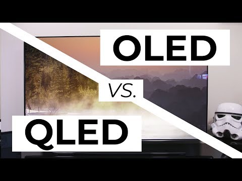
Supported by LG, Philips, Panasonic and Sony sell the OLED system TVs.
OLED stands for “organic light emitting diode.”
It is a fundamentally different technology from LCD, the major type of TV today.
OLED is “emissive,” meaning the pixels emit their own light.Samsung is branding its best TVs with a new acronym: “QLED”
QLED (according to Samsung) stands for “quantum dot LED TV.”
It is a variation of the common LED LCD, adding a quantum dot film to the LCD “sandwich.”
QLED, like LCD, is, in its current form, “transmissive” and relies on an LED backlight.OLED is the only technology capable of absolute blacks and extremely bright whites on a per-pixel basis. LCD definitely can’t do that, and even the vaunted, beloved, dearly departed plasma couldn’t do absolute blacks.
QLED, as an improvement over OLED, significantly improves the picture quality. QLED can produce an even wider range of colors than OLED, which says something about this new tech. QLED is also known to produce up to 40% higher luminance efficiency than OLED technology. Further, many tests conclude that QLED is far more efficient in terms of power consumption than its predecessor, OLED.
(more…) -
sRGB vs REC709 – An introduction and FFmpeg implementations
Read more: sRGB vs REC709 – An introduction and FFmpeg implementations
1. Basic Comparison
- What they are
- sRGB: A standard “web”/computer-display RGB color space defined by IEC 61966-2-1. It’s used for most monitors, cameras, printers, and the vast majority of images on the Internet.
- Rec. 709: An HD-video color space defined by ITU-R BT.709. It’s the go-to standard for HDTV broadcasts, Blu-ray discs, and professional video pipelines.
- Why they exist
- sRGB: Ensures consistent colors across different consumer devices (PCs, phones, webcams).
- Rec. 709: Ensures consistent colors across video production and playback chains (cameras → editing → broadcast → TV).
- What you’ll see
- On your desktop or phone, images tagged sRGB will look “right” without extra tweaking.
- On an HDTV or video-editing timeline, footage tagged Rec. 709 will display accurate contrast and hue on broadcast-grade monitors.
2. Digging Deeper
Feature sRGB Rec. 709 White point D65 (6504 K), same for both D65 (6504 K) Primaries (x,y) R: (0.640, 0.330) G: (0.300, 0.600) B: (0.150, 0.060) R: (0.640, 0.330) G: (0.300, 0.600) B: (0.150, 0.060) Gamut size Identical triangle on CIE 1931 chart Identical to sRGB Gamma / transfer Piecewise curve: approximate 2.2 with linear toe Pure power-law γ≈2.4 (often approximated as 2.2 in practice) Matrix coefficients N/A (pure RGB usage) Y = 0.2126 R + 0.7152 G + 0.0722 B (Rec. 709 matrix) Typical bit-depth 8-bit/channel (with 16-bit variants) 8-bit/channel (10-bit for professional video) Usage metadata Tagged as “sRGB” in image files (PNG, JPEG, etc.) Tagged as “bt709” in video containers (MP4, MOV) Color range Full-range RGB (0–255) Studio-range Y′CbCr (Y′ [16–235], Cb/Cr [16–240])
Why the Small Differences Matter
(more…) - What they are
-
Weta Digital – Manuka Raytracer and Gazebo GPU renderers – pipeline
Read more: Weta Digital – Manuka Raytracer and Gazebo GPU renderers – pipelinehttps://jo.dreggn.org/home/2018_manuka.pdf
http://www.fxguide.com/featured/manuka-weta-digitals-new-renderer/

The Manuka rendering architecture has been designed in the spirit of the classic reyes rendering architecture. In its core, reyes is based on stochastic rasterisation of micropolygons, facilitating depth of field, motion blur, high geometric complexity,and programmable shading.
This is commonly achieved with Monte Carlo path tracing, using a paradigm often called shade-on-hit, in which the renderer alternates tracing rays with running shaders on the various ray hits. The shaders take the role of generating the inputs of the local material structure which is then used bypath sampling logic to evaluate contributions and to inform what further rays to cast through the scene.
Over the years, however, the expectations have risen substantially when it comes to image quality. Computing pictures which are indistinguishable from real footage requires accurate simulation of light transport, which is most often performed using some variant of Monte Carlo path tracing. Unfortunately this paradigm requires random memory accesses to the whole scene and does not lend itself well to a rasterisation approach at all.
Manuka is both a uni-directional and bidirectional path tracer and encompasses multiple importance sampling (MIS). Interestingly, and importantly for production character skin work, it is the first major production renderer to incorporate spectral MIS in the form of a new ‘Hero Spectral Sampling’ technique, which was recently published at Eurographics Symposium on Rendering 2014.
Manuka propose a shade-before-hit paradigm in-stead and minimise I/O strain (and some memory costs) on the system, leveraging locality of reference by running pattern generation shaders before we execute light transport simulation by path sampling, “compressing” any bvh structure as needed, and as such also limiting duplication of source data.
The difference with reyes is that instead of baking colors into the geometry like in Reyes, manuka bakes surface closures. This means that light transport is still calculated with path tracing, but all texture lookups etc. are done up-front and baked into the geometry.The main drawback with this method is that geometry has to be tessellated to its highest, stable topology before shading can be evaluated properly. As such, the high cost to first pixel. Even a basic 4 vertices square becomes a much more complex model with this approach.

Manuka use the RenderMan Shading Language (rsl) for programmable shading [Pixar Animation Studios 2015], but we do not invoke rsl shaders when intersecting a ray with a surface (often called shade-on-hit). Instead, we pre-tessellate and pre-shade all the input geometry in the front end of the renderer.
This way, we can efficiently order shading computations to sup-port near-optimal texture locality, vectorisation, and parallelism. This system avoids repeated evaluation of shaders at the same surface point, and presents a minimal amount of memory to be accessed during light transport time. An added benefit is that the acceleration structure for ray tracing (abounding volume hierarchy, bvh) is built once on the final tessellated geometry, which allows us to ray trace more efficiently than multi-level bvhs and avoids costly caching of on-demand tessellated micropolygons and the associated scheduling issues.For the shading reasons above, in terms of AOVs, the studio approach is to succeed at combining complex shading with ray paths in the render rather than pass a multi-pass render to compositing.
For the Spectral Rendering component. The light transport stage is fully spectral, using a continuously sampled wavelength which is traced with each path and used to apply the spectral camera sensitivity of the sensor. This allows for faithfully support any degree of observer metamerism as the camera footage they are intended to match as well as complex materials which require wavelength dependent phenomena such as diffraction, dispersion, interference, iridescence, or chromatic extinction and Rayleigh scattering in participating media.
As opposed to the original reyes paper, we use bilinear interpolation of these bsdf inputs later when evaluating bsdfs per pathv ertex during light transport4. This improves temporal stability of geometry which moves very slowly with respect to the pixel raster
In terms of the pipeline, everything rendered at Weta was already completely interwoven with their deep data pipeline. Manuka very much was written with deep data in mind. Here, Manuka not so much extends the deep capabilities, rather it fully matches the already extremely complex and powerful setup Weta Digital already enjoy with RenderMan. For example, an ape in a scene can be selected, its ID is available and a NUKE artist can then paint in 3D say a hand and part of the way up the neutral posed ape.
We called our system Manuka, as a respectful nod to reyes: we had heard a story froma former ILM employee about how reyes got its name from how fond the early Pixar people were of their lunches at Point Reyes, and decided to name our system after our surrounding natural environment, too. Manuka is a kind of tea tree very common in New Zealand which has very many very small leaves, in analogy to micropolygons ina tree structure for ray tracing. It also happens to be the case that Weta Digital’s main site is on Manuka Street.

-
THOMAS MANSENCAL – The Apparent Simplicity of RGB Rendering
Read more: THOMAS MANSENCAL – The Apparent Simplicity of RGB Rendering
https://thomasmansencal.substack.com/p/the-apparent-simplicity-of-rgb-rendering
The primary goal of physically-based rendering (PBR) is to create a simulation that accurately reproduces the imaging process of electro-magnetic spectrum radiation incident to an observer. This simulation should be indistinguishable from reality for a similar observer.
Because a camera is not sensitive to incident light the same way than a human observer, the images it captures are transformed to be colorimetric. A project might require infrared imaging simulation, a portion of the electro-magnetic spectrum that is invisible to us. Radically different observers might image the same scene but the act of observing does not change the intrinsic properties of the objects being imaged. Consequently, the physical modelling of the virtual scene should be independent of the observer.
-
HDR and Color
Read more: HDR and Colorhttps://www.soundandvision.com/content/nits-and-bits-hdr-and-color
In HD we often refer to the range of available colors as a color gamut. Such a color gamut is typically plotted on a two-dimensional diagram, called a CIE chart, as shown in at the top of this blog. Each color is characterized by its x/y coordinates.

Good enough for government work, perhaps. But for HDR, with its higher luminance levels and wider color, the gamut becomes three-dimensional.

For HDR the color gamut therefore becomes a characteristic we now call the color volume. It isn’t easy to show color volume on a two-dimensional medium like the printed page or a computer screen, but one method is shown below. As the luminance becomes higher, the picture eventually turns to white. As it becomes darker, it fades to black. The traditional color gamut shown on the CIE chart is simply a slice through this color volume at a selected luminance level, such as 50%.
Three different color volumes—we still refer to them as color gamuts though their third dimension is important—are currently the most significant. The first is BT.709 (sometimes referred to as Rec.709), the color gamut used for pre-UHD/HDR formats, including standard HD.
The largest is known as BT.2020; it encompasses (roughly) the range of colors visible to the human eye (though ET might find it insufficient!).
Between these two is the color gamut used in digital cinema, known as DCI-P3.

sRGB

D65

-
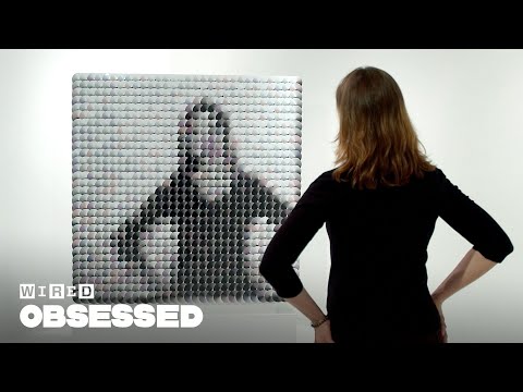
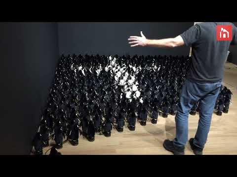
SecretWeapons MixBox – a practical library for paint-like digital color mixing
Read more: SecretWeapons MixBox – a practical library for paint-like digital color mixingInternally, Mixbox treats colors as real-life pigments using the Kubelka & Munk theory to predict realistic color behavior.
https://scrtwpns.com/mixbox/painter/
https://scrtwpns.com/mixbox.pdf
https://github.com/scrtwpns/mixbox
https://scrtwpns.com/mixbox/docs/


LIGHTING
-
DiffusionLight: HDRI Light Probes for Free by Painting a Chrome Ball
Read more: DiffusionLight: HDRI Light Probes for Free by Painting a Chrome Ballhttps://diffusionlight.github.io/
https://github.com/DiffusionLight/DiffusionLight
https://github.com/DiffusionLight/DiffusionLight?tab=MIT-1-ov-file#readme
https://colab.research.google.com/drive/15pC4qb9mEtRYsW3utXkk-jnaeVxUy-0S
“a simple yet effective technique to estimate lighting in a single input image. Current techniques rely heavily on HDR panorama datasets to train neural networks to regress an input with limited field-of-view to a full environment map. However, these approaches often struggle with real-world, uncontrolled settings due to the limited diversity and size of their datasets. To address this problem, we leverage diffusion models trained on billions of standard images to render a chrome ball into the input image. Despite its simplicity, this task remains challenging: the diffusion models often insert incorrect or inconsistent objects and cannot readily generate images in HDR format. Our research uncovers a surprising relationship between the appearance of chrome balls and the initial diffusion noise map, which we utilize to consistently generate high-quality chrome balls. We further fine-tune an LDR difusion model (Stable Diffusion XL) with LoRA, enabling it to perform exposure bracketing for HDR light estimation. Our method produces convincing light estimates across diverse settings and demonstrates superior generalization to in-the-wild scenarios.”

-
HDRI shooting and editing by Xuan Prada and Greg Zaal
Read more: HDRI shooting and editing by Xuan Prada and Greg Zaalwww.xuanprada.com/blog/2014/11/3/hdri-shooting
http://blog.gregzaal.com/2016/03/16/make-your-own-hdri/
http://blog.hdrihaven.com/how-to-create-high-quality-hdri/
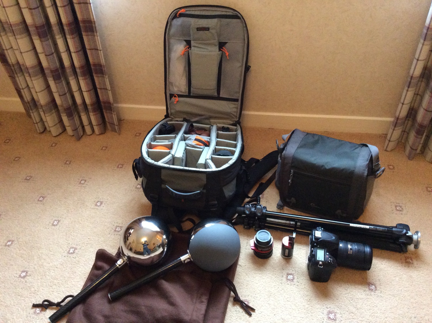
Shooting checklist
- Full coverage of the scene (fish-eye shots)
- Backplates for look-development (including ground or floor)
- Macbeth chart for white balance
- Grey ball for lighting calibration
- Chrome ball for lighting orientation
- Basic scene measurements
- Material samples
- Individual HDR artificial lighting sources if required
Methodology
(more…) -
Custom bokeh in a raytraced DOF render
Read more: Custom bokeh in a raytraced DOF render

To achieve a custom pinhole camera effect with a custom bokeh in Arnold Raytracer, you can follow these steps:
- Set the render camera with a focal length around 50 (or as needed)
- Set the F-Stop to a high value (e.g., 22).
- Set the focus distance as you require
- Turn on DOF
- Place a plane a few cm in front of the camera.
- Texture the plane with a transparent shape at the center of it. (Transmission with no specular roughness)


COLLECTIONS
| Featured AI
| Design And Composition
| Explore posts
POPULAR SEARCHES
unreal | pipeline | virtual production | free | learn | photoshop | 360 | macro | google | nvidia | resolution | open source | hdri | real-time | photography basics | nuke
FEATURED POSTS
-
Guide to Prompt Engineering
-
JavaScript how-to free resources
-
HoloCine – Holistic Generation of Cinematic Multi-Shot Long Video Narratives
-
AI and the Law – studiobinder.com – What is Fair Use: Definition, Policies, Examples and More
-
Emmanuel Tsekleves – Writing Research Papers
-
Convert 2D Images or Text to 3D Models
-
Photography basics: Production Rendering Resolution Charts
-
sRGB vs REC709 – An introduction and FFmpeg implementations
Social Links
DISCLAIMER – Links and images on this website may be protected by the respective owners’ copyright. All data submitted by users through this site shall be treated as freely available to share.
