


COMPOSITION
-
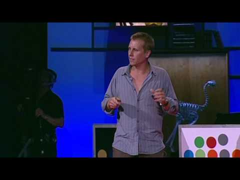
Mastering Camera Shots and Angles: A Guide for Filmmakers
Read more: Mastering Camera Shots and Angles: A Guide for Filmmakershttps://website.ltx.studio/blog/mastering-camera-shots-and-angles
1. Extreme Wide Shot

2. Wide Shot

3. Medium Shot

4. Close Up

5. Extreme Close Up


DESIGN
-
IM3 Stained glass
Read more: IM3 Stained glass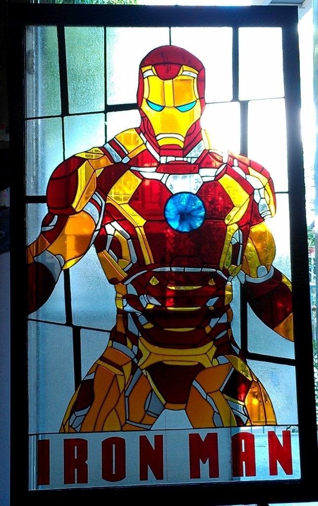
http://imgur.com/a/GXUun#hO6wzrs
Some people are asking how… here is a brief explanation on how I did it with photos….
(more…) -
Kelly Boesch – Static and Toward The Light
Read more: Kelly Boesch – Static and Toward The Lighthttps://www.kellyboeschdesign.com
I was working an album cover last night and got these really cool images in midjourney so made a video out of it. Animated using Pika. Song made using Suno Full version on my bandcamp. It’s called Static.
https://www.linkedin.com/posts/kellyboesch_midjourney-keyframes-ai-activity-7359244714853736450-Wvcr(more…)


COLOR
-
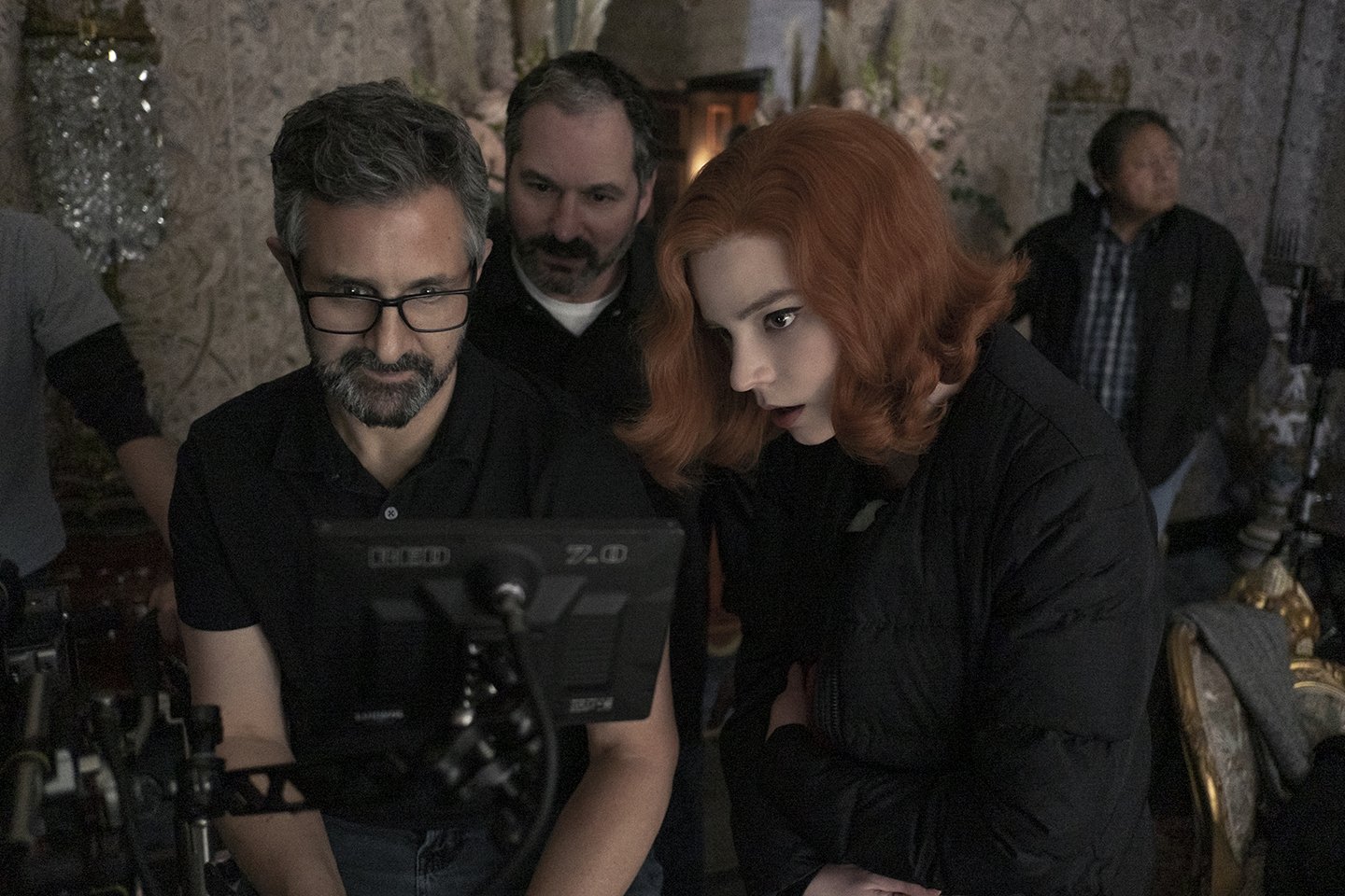
Colour – MacBeth Chart Checker Detection
Read more: Colour – MacBeth Chart Checker Detectiongithub.com/colour-science/colour-checker-detection
A Python package implementing various colour checker detection algorithms and related utilities.


LIGHTING
-
Lighting Every Darkness with 3DGS: Fast Training and Real-Time Rendering and Denoising for HDR View Synthesis
Read more: Lighting Every Darkness with 3DGS: Fast Training and Real-Time Rendering and Denoising for HDR View Synthesishttps://srameo.github.io/projects/le3d/
LE3D is a method for real-time HDR view synthesis from RAW images. It is particularly effective for nighttime scenes.
https://github.com/Srameo/LE3D


-
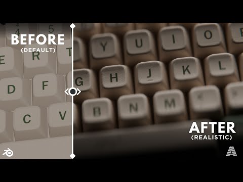
Bella – Fast Spectral Rendering
Read more: Bella – Fast Spectral Rendering
Bella works in spectral space, allowing effects such as BSDF wavelength dependency, diffraction, or atmosphere to be modeled far more accurately than in color space.

https://superrendersfarm.com/blog/uncategorized/bella-a-new-spectral-physically-based-renderer/
-
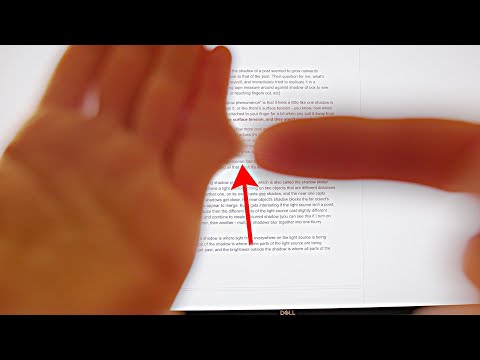
Photography basics: Lumens vs Candelas (candle) vs Lux vs FootCandle vs Watts vs Irradiance vs Illuminance
Read more: Photography basics: Lumens vs Candelas (candle) vs Lux vs FootCandle vs Watts vs Irradiance vs Illuminancehttps://www.translatorscafe.com/unit-converter/en-US/illumination/1-11/

The power output of a light source is measured using the unit of watts W. This is a direct measure to calculate how much power the light is going to drain from your socket and it is not relatable to the light brightness itself.
The amount of energy emitted from it per second. That energy comes out in a form of photons which we can crudely represent with rays of light coming out of the source. The higher the power the more rays emitted from the source in a unit of time.
Not all energy emitted is visible to the human eye, so we often rely on photometric measurements, which takes in account the sensitivity of human eye to different wavelenghts


Details in the post
(more…)


COLLECTIONS
| Featured AI
| Design And Composition
| Explore posts
POPULAR SEARCHES
unreal | pipeline | virtual production | free | learn | photoshop | 360 | macro | google | nvidia | resolution | open source | hdri | real-time | photography basics | nuke
FEATURED POSTS
-
VFX pipeline – Render Wall Farm management topics
-
Photography basics: Shutter angle and shutter speed and motion blur
-
59 AI Filmmaking Tools For Your Workflow
-
Tencent Hunyuan3D 2.1 goes Open Source and adds MV (Multi-view) and MV Mini
-
Photography basics: Production Rendering Resolution Charts
-
Animation/VFX/Game Industry JOB POSTINGS by Chris Mayne
-
Alejandro Villabón and Rafał Kaniewski – Recover Highlights With 8-Bit to High Dynamic Range Half Float Copycat – Nuke
-
Ethan Roffler interviews CG Supervisor Daniele Tosti
Social Links
DISCLAIMER – Links and images on this website may be protected by the respective owners’ copyright. All data submitted by users through this site shall be treated as freely available to share.
