


COMPOSITION
-
HuggingFace ai-comic-factory – a FREE AI Comic Book Creator
Read more: HuggingFace ai-comic-factory – a FREE AI Comic Book Creatorhttps://huggingface.co/spaces/jbilcke-hf/ai-comic-factory

this is the epic story of a group of talented digital artists trying to overcame daily technical challenges to achieve incredibly photorealistic projects of monsters and aliens


DESIGN
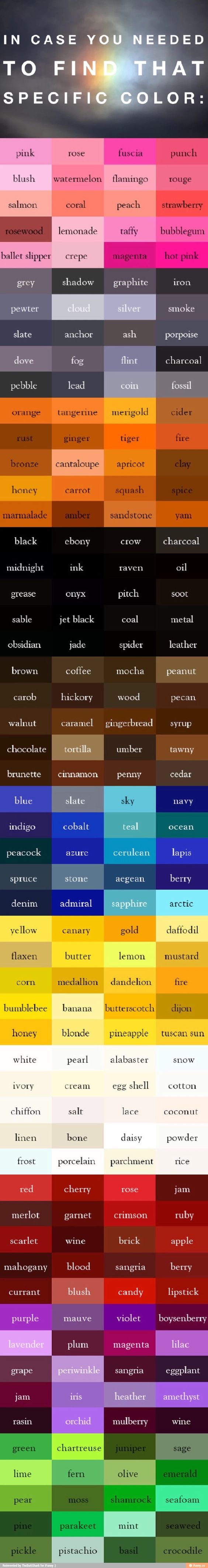
COLOR
-
About color: What is a LUT
Read more: About color: What is a LUThttp://www.lightillusion.com/luts.html
https://www.shutterstock.com/blog/how-use-luts-color-grading
A LUT (Lookup Table) is essentially the modifier between two images, the original image and the displayed image, based on a mathematical formula. Basically conversion matrices of different complexities. There are different types of LUTS – viewing, transform, calibration, 1D and 3D.


-
Anders Langlands – Render Color Spaces
Read more: Anders Langlands – Render Color Spaceshttps://www.colour-science.org/anders-langlands/
This page compares images rendered in Arnold using spectral rendering and different sets of colourspace primaries: Rec.709, Rec.2020, ACES and DCI-P3. The SPD data for the GretagMacbeth Color Checker are the measurements of Noburu Ohta, taken from Mansencal, Mauderer and Parsons (2014) colour-science.org.

-
GretagMacbeth Color Checker Numeric Values and Middle Gray
Read more: GretagMacbeth Color Checker Numeric Values and Middle GrayThe human eye perceives half scene brightness not as the linear 50% of the present energy (linear nature values) but as 18% of the overall brightness. We are biased to perceive more information in the dark and contrast areas. A Macbeth chart helps with calibrating back into a photographic capture into this “human perspective” of the world.
https://en.wikipedia.org/wiki/Middle_gray
In photography, painting, and other visual arts, middle gray or middle grey is a tone that is perceptually about halfway between black and white on a lightness scale in photography and printing, it is typically defined as 18% reflectance in visible light

Light meters, cameras, and pictures are often calibrated using an 18% gray card[4][5][6] or a color reference card such as a ColorChecker. On the assumption that 18% is similar to the average reflectance of a scene, a grey card can be used to estimate the required exposure of the film.
https://en.wikipedia.org/wiki/ColorChecker
(more…) -
Virtual Production volumes study
Read more: Virtual Production volumes studyColor Fidelity in LED Volumes
https://theasc.com/articles/color-fidelity-in-led-volumes
Virtual Production Glossary
https://vpglossary.com/What is Virtual Production – In depth analysis
https://www.leadingledtech.com/what-is-a-led-virtual-production-studio-in-depth-technical-analysis/
A comparison of LED panels for use in Virtual Production:
Findings and recommendations
https://eprints.bournemouth.ac.uk/36826/1/LED_Comparison_White_Paper%281%29.pdf


LIGHTING
-
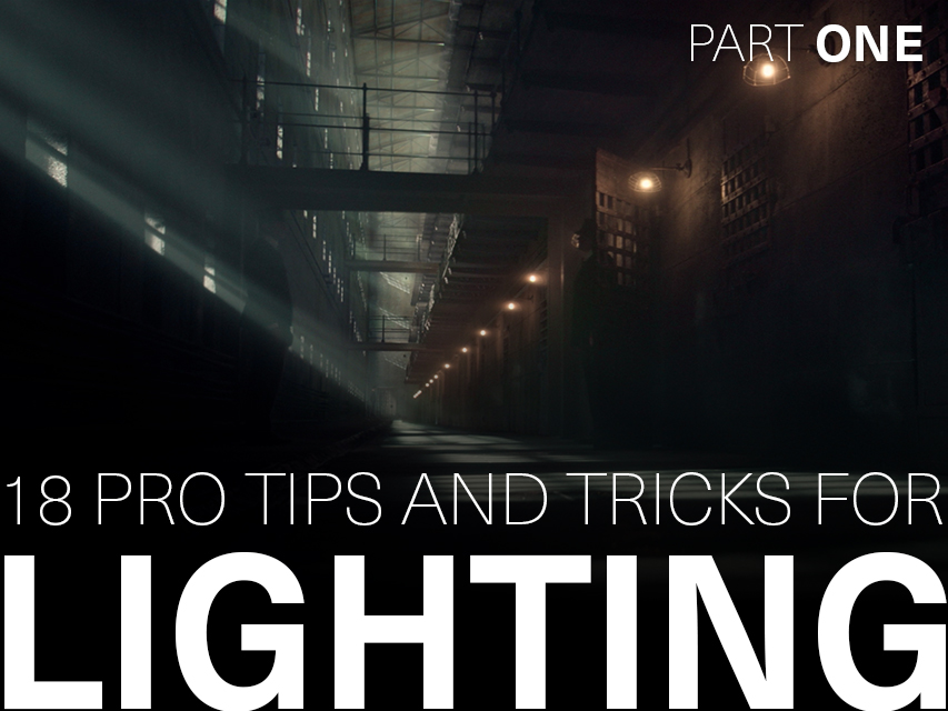
Outpost VFX lighting tips
Read more: Outpost VFX lighting tipswww.outpost-vfx.com/en/news/18-pro-tips-and-tricks-for-lighting
Get as much information regarding your plate lighting as possible
- Always use a reference
- Replicate what is happening in real life
- Invest into a solid HDRI
- Start Simple
- Observe real world lighting, photography and cinematography
- Don’t neglect the theory
- Learn the difference between realism and photo-realism.
- Keep your scenes organised
-
Sun cone angle (angular diameter) as perceived by earth viewers
Read more: Sun cone angle (angular diameter) as perceived by earth viewersAlso see:
https://www.pixelsham.com/2020/08/01/solid-angle-measures/
The cone angle of the sun refers to the angular diameter of the sun as observed from Earth, which is related to the apparent size of the sun in the sky.
The angular diameter of the sun, or the cone angle of the sunlight as perceived from Earth, is approximately 0.53 degrees on average. This value can vary slightly due to the elliptical nature of Earth’s orbit around the sun, but it generally stays within a narrow range.
Here’s a more precise breakdown:
-
- Average Angular Diameter: About 0.53 degrees (31 arcminutes)
- Minimum Angular Diameter: Approximately 0.52 degrees (when Earth is at aphelion, the farthest point from the sun)
- Maximum Angular Diameter: Approximately 0.54 degrees (when Earth is at perihelion, the closest point to the sun)
This angular diameter remains relatively constant throughout the day because the sun’s distance from Earth does not change significantly over a single day.
To summarize, the cone angle of the sun’s light, or its angular diameter, is typically around 0.53 degrees, regardless of the time of day.
https://en.wikipedia.org/wiki/Angular_diameter

-
-
Disney’s Moana Island Scene – Free data set
Read more: Disney’s Moana Island Scene – Free data sethttps://www.disneyanimation.com/resources/moana-island-scene/
This data set contains everything necessary to render a version of the Motunui island featured in the 2016 film Moana.


COLLECTIONS
| Featured AI
| Design And Composition
| Explore posts
POPULAR SEARCHES
unreal | pipeline | virtual production | free | learn | photoshop | 360 | macro | google | nvidia | resolution | open source | hdri | real-time | photography basics | nuke
FEATURED POSTS
-
Types of AI Explained in a few Minutes – AI Glossary
-
How to paint a boardgame miniatures
-
How does Stable Diffusion work?
-
Most common ways to smooth 3D prints
-
How do LLMs like ChatGPT (Generative Pre-Trained Transformer) work? Explained by Deep-Fake Ryan Gosling
-
Photography basics: Solid Angle measures
-
sRGB vs REC709 – An introduction and FFmpeg implementations
-
Top 3D Printing Website Resources
Social Links
DISCLAIMER – Links and images on this website may be protected by the respective owners’ copyright. All data submitted by users through this site shall be treated as freely available to share.
