Depth of field is the range within which focusing is resolved in a photo.
Aperture has a huge affect on to the depth of field.
Changing the f-stops (f/#) of a lens will change aperture and as such the DOF.
f-stops are a just certain number which is telling you the size of the aperture. That’s how f-stop is related to aperture (and DOF).
If you increase f-stops, it will increase DOF, the area in focus (and decrease the aperture). On the other hand, decreasing the f-stop it will decrease DOF (and increase the aperture).
The red cone in the figure is an angular representation of the resolution of the system. Versus the dotted lines, which indicate the aperture coverage. Where the lines of the two cones intersect defines the total range of the depth of field.
This image explains why the longer the depth of field, the greater the range of clarity.
This demo is created for coders who are familiar with this awesome creative coding platform. You may quickly modify the code to work for video or to stipple your own Procssing drawings by turning them into PImage and run the simulation. This demo code also serves as a reference implementation of my article Blue noise sampling using an N-body simulation-based method. If you are interested in 2.5D, you may mod the code to achieve what I discussed in this artist friendly article.
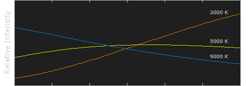
Black-body radiation is the type of electromagnetic radiation within or surrounding a body in thermodynamic equilibrium with its environment, or emitted by a black body (an opaque and non-reflective body) held at constant, uniform temperature. The radiation has a specific spectrum and intensity that depends only on the temperature of the body.
A black-body at room temperature appears black, as most of the energy it radiates is infra-red and cannot be perceived by the human eye. At higher temperatures, black bodies glow with increasing intensity and colors that range from dull red to blindingly brilliant blue-white as the temperature increases.
The Black Body Ultraviolet Catastrophe Experiment
In photography, color temperature describes the spectrum of light which is radiated from a “blackbody” with that surface temperature. A blackbody is an object which absorbs all incident light — neither reflecting it nor allowing it to pass through.
The Sun closely approximates a black-body radiator. Another rough analogue of blackbody radiation in our day to day experience might be in heating a metal or stone: these are said to become “red hot” when they attain one temperature, and then “white hot” for even higher temperatures. Similarly, black bodies at different temperatures also have varying color temperatures of “white light.”
Despite its name, light which may appear white does not necessarily contain an even distribution of colors across the visible spectrum.
Although planets and stars are neither in thermal equilibrium with their surroundings nor perfect black bodies, black-body radiation is used as a first approximation for the energy they emit. Black holes are near-perfect black bodies, and it is believed that they emit black-body radiation (called Hawking radiation), with a temperature that depends on the mass of the hole.
In color technology, color depth also known as bit depth, is either the number of bits used to indicate the color of a single pixel, OR the number of bits used for each color component of a single pixel.
When referring to a pixel, the concept can be defined as bits per pixel (bpp).
When referring to a color component, the concept can be defined as bits per component, bits per channel, bits per color (all three abbreviated bpc), and also bits per pixel component, bits per color channel or bits per sample (bps). Modern standards tend to use bits per component, but historical lower-depth systems used bits per pixel more often.
Color depth is only one aspect of color representation, expressing the precision with which the amount of each primary can be expressed; the other aspect is how broad a range of colors can be expressed (the gamut). The definition of both color precision and gamut is accomplished with a color encoding specification which assigns a digital code value to a location in a color space.
ACES 2.0 is the second major release of the components that make up the ACES system. The most significant change is a new suite of rendering transforms whose design was informed by collected feedback and requests from users of ACES 1. The changes aim to improve the appearance of perceived artifacts and to complete previously unfinished components of the system, resulting in a more complete, robust, and consistent product.
Highlights of the key changes in ACES 2.0 are as follows:
New output transforms, including:
A less aggressive tone scale
More intuitive controls to create custom outputs to non-standard displays
Robust gamut mapping to improve perceptual uniformity
Improved performance of the inverse transforms
Enhanced AMF specification
An updated specification for ACES Transform IDs
OpenEXR compression recommendations
Enhanced tools for generating Input Transforms and recommended procedures for characterizing prosumer cameras
Look Transform Library
Expanded documentation
Rendering Transform
The most substantial change in ACES 2.0 is a complete redesign of the rendering transform.
ACES 2.0 was built as a unified system, rather than through piecemeal additions. Different deliverable outputs “match” better and making outputs to display setups other than the provided presets is intended to be user-driven. The rendering transforms are less likely to produce undesirable artifacts “out of the box”, which means less time can be spent fixing problematic images and more time making pictures look the way you want.
Key design goals
Improve consistency of tone scale and provide an easy to use parameter to allow for outputs between preset dynamic ranges
Minimize hue skews across exposure range in a region of same hue
Unify for structural consistency across transform type
Easy to use parameters to create outputs other than the presets
Robust gamut mapping to improve harsh clipping artifacts
Fill extents of output code value cube (where appropriate and expected)
Invertible – not necessarily reversible, but Output > ACES > Output round-trip should be possible
Accomplish all of the above while maintaining an acceptable “out-of-the box” rendering
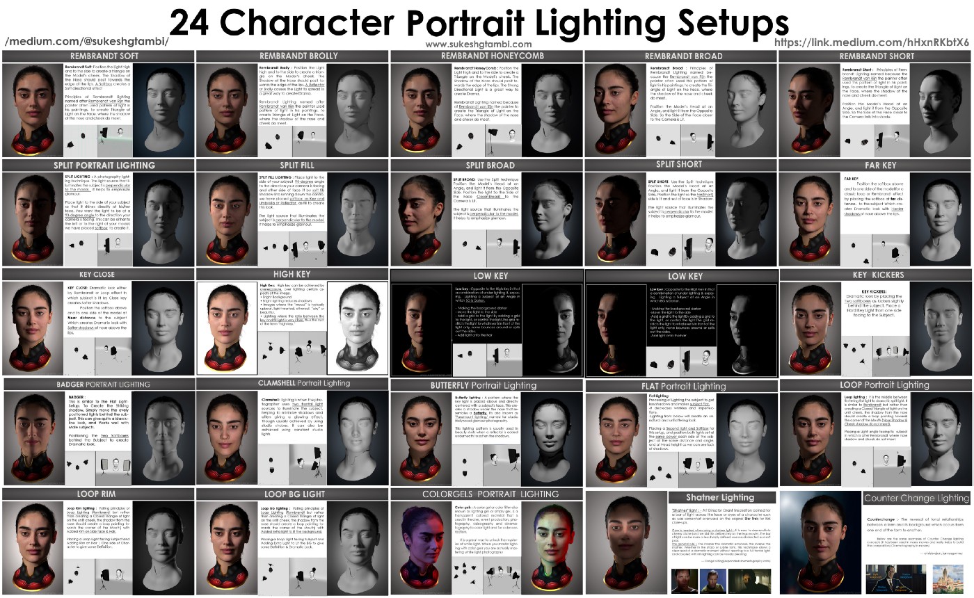
The goals of lighting in 3D computer graphics are more or less the same as those of real world lighting.
Lighting serves a basic function of bringing out, or pushing back the shapes of objects visible from the camera’s view.
It gives a two-dimensional image on the monitor an illusion of the third dimension-depth.
But it does not just stop there. It gives an image its personality, its character. A scene lit in different ways can give a feeling of happiness, of sorrow, of fear etc., and it can do so in dramatic or subtle ways. Along with personality and character, lighting fills a scene with emotion that is directly transmitted to the viewer.
Trying to simulate a real environment in an artificial one can be a daunting task. But even if you make your 3D rendering look absolutely photo-realistic, it doesn’t guarantee that the image carries enough emotion to elicit a “wow” from the people viewing it.
Making 3D renderings photo-realistic can be hard. Putting deep emotions in them can be even harder. However, if you plan out your lighting strategy for the mood and emotion that you want your rendering to express, you make the process easier for yourself.
Each light source can be broken down in to 4 distinct components and analyzed accordingly.
· Intensity
· Direction
· Color
· Size
The overall thrust of this writing is to produce photo-realistic images by applying good lighting techniques.
Size. Mr. White (Harvey Keitel) on the right. Focus. He’s one of the two objects in focus. Lighting. Mr. White is large and in focus and Mr. Pink (Steve Buscemi) is highlighted by a shaft of light. Color. Both are black and white but the read on Mr. White’s shirt now really stands out.
Note: In Foundry’s Nuke, the software will map 18% gray to whatever your center f/stop is set to in the viewer settings (f/8 by default… change that to EV by following the instructions below).
You can experiment with this by attaching an Exposure node to a Constant set to 0.18, setting your viewer read-out to Spotmeter, and adjusting the stops in the node up and down. You will see that a full stop up or down will give you the respective next value on the aperture scale (f8, f11, f16 etc.).
One stop doubles or halves the amount or light that hits the filmback/ccd, so everything works in powers of 2.
So starting with 0.18 in your constant, you will see that raising it by a stop will give you .36 as a floating point number (in linear space), while your f/stop will be f/11 and so on.
If you set your center stop to 0 (see below) you will get a relative readout in EVs, where EV 0 again equals 18% constant gray.
In other words. Setting the center f-stop to 0 means that in a neutral plate, the middle gray in the macbeth chart will equal to exposure value 0. EV 0 corresponds to an exposure time of 1 sec and an aperture of f/1.0.
This will set the sun usually around EV12-17 and the sky EV1-4 , depending on cloud coverage.
To switch Foundry’s Nuke’s SpotMeter to return the EV of an image, click on the main viewport, and then press s, this opens the viewer’s properties. Now set the center f-stop to 0 in there. And the SpotMeter in the viewport will change from aperture and fstops to EV.
DISCLAIMER – Links and images on this website may be protected by the respective owners’ copyright. All data submitted by users through this site shall be treated as freely available to share.


 Local copy: