To measure the contrast ratio you will need a light meter. The process starts with you measuring the main source of light, or the key light.
Get a reading from the brightest area on the face of your subject. Then, measure the area lit by the secondary light, or fill light. To make sense of what you have just measured you have to understand that the information you have just gathered is in F-stops, a measure of light. With each additional F-stop, for example going one stop from f/1.4 to f/2.0, you create a doubling of light. The reverse is also true; moving one stop from f/8.0 to f/5.6 results in a halving of the light.
this is the epic story of a group of talented digital artists trying to overcame daily technical challenges to achieve incredibly photorealistic projects of monsters and aliens
A number of problems in computer vision and related fields would be mitigated if camera spectral sensitivities were known. As consumer cameras are not designed for high-precision visual tasks, manufacturers do not disclose spectral sensitivities. Their estimation requires a costly optical setup, which triggered researchers to come up with numerous indirect methods that aim to lower cost and complexity by using color targets. However, the use of color targets gives rise to new complications that make the estimation more difficult, and consequently, there currently exists no simple, low-cost, robust go-to method for spectral sensitivity estimation that non-specialized research labs can adopt. Furthermore, even if not limited by hardware or cost, researchers frequently work with imagery from multiple cameras that they do not have in their possession.
To provide a practical solution to this problem, we propose a framework for spectral sensitivity estimation that not only does not require any hardware (including a color target), but also does not require physical access to the camera itself. Similar to other work, we formulate an optimization problem that minimizes a two-term objective function: a camera-specific term from a system of equations, and a universal term that bounds the solution space.
Different than other work, we utilize publicly available high-quality calibration data to construct both terms. We use the colorimetric mapping matrices provided by the Adobe DNG Converter to formulate the camera-specific system of equations, and constrain the solutions using an autoencoder trained on a database of ground-truth curves. On average, we achieve reconstruction errors as low as those that can arise due to manufacturing imperfections between two copies of the same camera. We provide predicted sensitivities for more than 1,000 cameras that the Adobe DNG Converter currently supports, and discuss which tasks can become trivial when camera responses are available.
Note: In Foundry’s Nuke, the software will map 18% gray to whatever your center f/stop is set to in the viewer settings (f/8 by default… change that to EV by following the instructions below).
You can experiment with this by attaching an Exposure node to a Constant set to 0.18, setting your viewer read-out to Spotmeter, and adjusting the stops in the node up and down. You will see that a full stop up or down will give you the respective next value on the aperture scale (f8, f11, f16 etc.).
One stop doubles or halves the amount or light that hits the filmback/ccd, so everything works in powers of 2.
So starting with 0.18 in your constant, you will see that raising it by a stop will give you .36 as a floating point number (in linear space), while your f/stop will be f/11 and so on.
If you set your center stop to 0 (see below) you will get a relative readout in EVs, where EV 0 again equals 18% constant gray.
In other words. Setting the center f-stop to 0 means that in a neutral plate, the middle gray in the macbeth chart will equal to exposure value 0. EV 0 corresponds to an exposure time of 1 sec and an aperture of f/1.0.
This will set the sun usually around EV12-17 and the sky EV1-4 , depending on cloud coverage.
To switch Foundry’s Nuke’s SpotMeter to return the EV of an image, click on the main viewport, and then press s, this opens the viewer’s properties. Now set the center f-stop to 0 in there. And the SpotMeter in the viewport will change from aperture and fstops to EV.
By stimulating specific cells in the retina, the participants claim to have witnessed a blue-green colour that scientists have called “olo”, but some experts have said the existence of a new colour is “open to argument”.
The findings, published in the journal Science Advances on Friday, have been described by the study’s co-author, Prof Ren Ng from the University of California, as “remarkable”.
(A) System inputs. (i) Retina map of 103 cone cells preclassified by spectral type (7). (ii) Target visual percept (here, a video of a child, see movie S1 at 1:04). (iii) Infrared cellular-scale imaging of the retina with 60-frames-per-second rolling shutter. Fixational eye movement is visible over the three frames shown.
(B) System outputs. (iv) Real-time per-cone target activation levels to reproduce the target percept, computed by: extracting eye motion from the input video relative to the retina map; identifying the spectral type of every cone in the field of view; computing the per-cone activation the target percept would have produced. (v) Intensities of visible-wavelength 488-nm laser microdoses at each cone required to achieve its target activation level.
(C) Infrared imaging and visible-wavelength stimulation are physically accomplished in a raster scan across the retinal region using AOSLO. By modulating the visible-wavelength beam’s intensity, the laser microdoses shown in (v) are delivered. Drawing adapted with permission [Harmening and Sincich (54)].
(D) Examples of target percepts with corresponding cone activations and laser microdoses, ranging from colored squares to complex imagery. Teal-striped regions represent the color “olo” of stimulating only M cones.
ACES 2.0 is the second major release of the components that make up the ACES system. The most significant change is a new suite of rendering transforms whose design was informed by collected feedback and requests from users of ACES 1. The changes aim to improve the appearance of perceived artifacts and to complete previously unfinished components of the system, resulting in a more complete, robust, and consistent product.
Highlights of the key changes in ACES 2.0 are as follows:
New output transforms, including:
A less aggressive tone scale
More intuitive controls to create custom outputs to non-standard displays
Robust gamut mapping to improve perceptual uniformity
Improved performance of the inverse transforms
Enhanced AMF specification
An updated specification for ACES Transform IDs
OpenEXR compression recommendations
Enhanced tools for generating Input Transforms and recommended procedures for characterizing prosumer cameras
Look Transform Library
Expanded documentation
Rendering Transform
The most substantial change in ACES 2.0 is a complete redesign of the rendering transform.
ACES 2.0 was built as a unified system, rather than through piecemeal additions. Different deliverable outputs “match” better and making outputs to display setups other than the provided presets is intended to be user-driven. The rendering transforms are less likely to produce undesirable artifacts “out of the box”, which means less time can be spent fixing problematic images and more time making pictures look the way you want.
Key design goals
Improve consistency of tone scale and provide an easy to use parameter to allow for outputs between preset dynamic ranges
Minimize hue skews across exposure range in a region of same hue
Unify for structural consistency across transform type
Easy to use parameters to create outputs other than the presets
Robust gamut mapping to improve harsh clipping artifacts
Fill extents of output code value cube (where appropriate and expected)
Invertible – not necessarily reversible, but Output > ACES > Output round-trip should be possible
Accomplish all of the above while maintaining an acceptable “out-of-the box” rendering
Blind people who regain their sight may find themselves in a world they don’t immediately comprehend. “It would be more like a sighted person trying to rely on tactile information,” Moore says.
Learning to see is a developmental process, just like learning language, Prof Cathleen Moore continues. “As far as vision goes, a three-and-a-half year old child is already a well-calibrated system.”
In HD we often refer to the range of available colors as a color gamut. Such a color gamut is typically plotted on a two-dimensional diagram, called a CIE chart, as shown in at the top of this blog. Each color is characterized by its x/y coordinates.
Good enough for government work, perhaps. But for HDR, with its higher luminance levels and wider color, the gamut becomes three-dimensional.
For HDR the color gamut therefore becomes a characteristic we now call the color volume. It isn’t easy to show color volume on a two-dimensional medium like the printed page or a computer screen, but one method is shown below. As the luminance becomes higher, the picture eventually turns to white. As it becomes darker, it fades to black. The traditional color gamut shown on the CIE chart is simply a slice through this color volume at a selected luminance level, such as 50%.
Three different color volumes—we still refer to them as color gamuts though their third dimension is important—are currently the most significant. The first is BT.709 (sometimes referred to as Rec.709), the color gamut used for pre-UHD/HDR formats, including standard HD.
The largest is known as BT.2020; it encompasses (roughly) the range of colors visible to the human eye (though ET might find it insufficient!).
Between these two is the color gamut used in digital cinema, known as DCI-P3.
A LUT (Lookup Table) is essentially the modifier between two images, the original image and the displayed image, based on a mathematical formula. Basically conversion matrices of different complexities. There are different types of LUTS – viewing, transform, calibration, 1D and 3D.
“Unless you have all the relevant spectral measurements, a colour rendition chart should not be used to perform colour-correction of camera imagery but only for white balancing and relative exposure adjustments.”
“Using a colour rendition chart for colour-correction might dramatically increase error if the scene light source spectrum is different from the illuminant used to compute the colour rendition chart’s reference values.”
“other factors make using a colour rendition chart unsuitable for camera calibration:
– Uncontrolled geometry of the colour rendition chart with the incident illumination and the camera.
– Unknown sample reflectances and ageing as the colour of the samples vary with time.
– Low samples count.
– Camera noise and flare.
– Etc…
“Those issues are well understood in the VFX industry, and when receiving plates, we almost exclusively use colour rendition charts to white balance and perform relative exposure adjustments, i.e. plate neutralisation.”
import math,sys

def Exposure2Intensity(exposure):
    exp = float(exposure)
    result = math.pow(2,exp)
    print(result)

Exposure2Intensity(0)

def Intensity2Exposure(intensity):
    inarg = float(intensity)

    if inarg == 0:
        print("Exposure of zero intensity is undefined.")
        return

    if inarg < 1e-323:
        inarg = max(inarg, 1e-323)
        print("Exposure of negative intensities is undefined. Clamping to a very small value instead (1e-323)")

    result = math.log(inarg, 2)
    print(result)

Intensity2Exposure(0.1)
Why Exposure?
Exposure is a stop value that multiplies the intensity by 2 to the power of the stop. Increasing exposure by 1 results in double the amount of light.
Artists think in “stops.” Doubling or halving brightness is easy math and common in grading and look-dev. Exposure counts doublings in whole stops:
+1 stop = ×2 brightness
−1 stop = ×0.5 brightness
This gives perceptually even controls across both bright and dark values.
Why Intensity?
Intensity is linear. It’s what render engines and compositors expect when:
Summing values
Averaging pixels
Multiplying or filtering pixel data
Use intensity when you need the actual math on pixel/light data.
Formulas (from your Python)
Intensity from exposure: intensity = 2**exposure
Exposure from intensity: exposure = log₂(intensity)
Guardrails:
Intensity must be > 0 to compute exposure.
If intensity = 0 → exposure is undefined.
Clamp tiny values (e.g. 1e−323) before using log₂.
Use Exposure (stops) when…
You want artist-friendly sliders (−5…+5 stops)
Adjusting look-dev or grading in even stops
Matching plates with quick ±1 stop tweaks
Tweening brightness changes smoothly across ranges
Use Intensity (linear) when…
Storing raw pixel/light values
Multiplying textures or lights by a gain
Performing sums, averages, and filters
Feeding values to render engines expecting linear data
Examples
+2 stops → 2**2 = 4.0 (×4)
+1 stop → 2**1 = 2.0 (×2)
0 stop → 2**0 = 1.0 (×1)
−1 stop → 2**(−1) = 0.5 (×0.5)
−2 stops → 2**(−2) = 0.25 (×0.25)
Intensity 0.1 → exposure = log₂(0.1) ≈ −3.32
Rule of thumb
Think in stops (exposure) for controls and matching. Compute in linear (intensity) for rendering and math.
The dynamic range is a ratio between the maximum and minimum values of a physical measurement. Its definition depends on what the dynamic range refers to.
For a scene: Dynamic range is the ratio between the brightest and darkest parts of the scene.
For a camera: Dynamic range is the ratio of saturation to noise. More specifically, the ratio of the intensity that just saturates the camera to the intensity that just lifts the camera response one standard deviation above camera noise.
For a display: Dynamic range is the ratio between the maximum and minimum intensities emitted from the screen.
The Dynamic Range of real-world scenes can be quite high — ratios of 100,000:1 are common in the natural world. An HDR (High Dynamic Range) image stores pixel values that span the whole tonal range of real-world scenes. Therefore, an HDR image is encoded in a format that allows the largest range of values, e.g. floating-point values stored with 32 bits per color channel. Another characteristics of an HDR image is that it stores linear values. This means that the value of a pixel from an HDR image is proportional to the amount of light measured by the camera.
For TVs HDR is great, but it’s not the only new TV feature worth discussing.
Ethan Roffler I recently had the honor of interviewing this VFX genius and gained great insight into what it takes to work in the entertainment industry. Keep in mind, these questions are coming from an artist’s perspective but can be applied to any creative individual looking for some wisdom from a professional. So grab a drink, sit back, and enjoy this fun and insightful conversation.
Ethan To start, I just wanted to say thank you so much for taking the time for this interview!
Daniele My pleasure. When I started my career I struggled to find help. Even people in the industry at the time were not that helpful. Because of that, I decided very early on that I was going to do exactly the opposite. I spend most of my weekends talking or helping students. ;)
Ethan That’s awesome! I have also come across the same struggle! Just a heads up, this will probably be the most informal interview you’ll ever have haha! Okay, so let’s start with a small introduction!
DISCLAIMER – Links and images on this website may be protected by the respective owners’ copyright. All data submitted by users through this site shall be treated as freely available to share.