this is the epic story of a group of talented digital artists trying to overcame daily technical challenges to achieve incredibly photorealistic projects of monsters and aliens
Of all the pigments that have been banned over the centuries, the color most missed by painters is likely Lead White.
This hue could capture and reflect a gleam of light like no other, though its production was anything but glamorous. The 17th-century Dutch method for manufacturing the pigment involved layering cow and horse manure over lead and vinegar. After three months in a sealed room, these materials would combine to create flakes of pure white. While scientists in the late 19th century identified lead as poisonous, it wasn’t until 1978 that the United States banned the production of lead white paint.
The dynamic range is a ratio between the maximum and minimum values of a physical measurement. Its definition depends on what the dynamic range refers to.
For a scene: Dynamic range is the ratio between the brightest and darkest parts of the scene.
For a camera: Dynamic range is the ratio of saturation to noise. More specifically, the ratio of the intensity that just saturates the camera to the intensity that just lifts the camera response one standard deviation above camera noise.
For a display: Dynamic range is the ratio between the maximum and minimum intensities emitted from the screen.
The Dynamic Range of real-world scenes can be quite high — ratios of 100,000:1 are common in the natural world. An HDR (High Dynamic Range) image stores pixel values that span the whole tonal range of real-world scenes. Therefore, an HDR image is encoded in a format that allows the largest range of values, e.g. floating-point values stored with 32 bits per color channel. Another characteristics of an HDR image is that it stores linear values. This means that the value of a pixel from an HDR image is proportional to the amount of light measured by the camera.
For TVs HDR is great, but it’s not the only new TV feature worth discussing.
In HD we often refer to the range of available colors as a color gamut. Such a color gamut is typically plotted on a two-dimensional diagram, called a CIE chart, as shown in at the top of this blog. Each color is characterized by its x/y coordinates.
Good enough for government work, perhaps. But for HDR, with its higher luminance levels and wider color, the gamut becomes three-dimensional.
For HDR the color gamut therefore becomes a characteristic we now call the color volume. It isn’t easy to show color volume on a two-dimensional medium like the printed page or a computer screen, but one method is shown below. As the luminance becomes higher, the picture eventually turns to white. As it becomes darker, it fades to black. The traditional color gamut shown on the CIE chart is simply a slice through this color volume at a selected luminance level, such as 50%.
Three different color volumes—we still refer to them as color gamuts though their third dimension is important—are currently the most significant. The first is BT.709 (sometimes referred to as Rec.709), the color gamut used for pre-UHD/HDR formats, including standard HD.
The largest is known as BT.2020; it encompasses (roughly) the range of colors visible to the human eye (though ET might find it insufficient!).
Between these two is the color gamut used in digital cinema, known as DCI-P3.
One problem with sRGB is that in a gradient between blue and white, it becomes a bit purple in the middle of the transition. That’s because sRGB really isn’t created to mimic how the eye sees colors; rather, it is based on how CRT monitors work. That means it works with certain frequencies of red, green, and blue, and also the non-linear coding called gamma. It’s a miracle it works as well as it does, but it’s not connected to color perception. When using those tools, you sometimes get surprising results, like purple in the gradient.
There were also attempts to create simple models matching human perception based on XYZ, but as it turned out, it’s not possible to model all color vision that way. Perception of color is incredibly complex and depends, among other things, on whether it is dark or light in the room and the background color it is against. When you look at a photograph, it also depends on what you think the color of the light source is. The dress is a typical example of color vision being very context-dependent. It is almost impossible to model this perfectly.
I based Oklab on two other color spaces, CIECAM16 and IPT. I used the lightness and saturation prediction from CIECAM16, which is a color appearance model, as a target. I actually wanted to use the datasets used to create CIECAM16, but I couldn’t find them.
IPT was designed to have better hue uniformity. In experiments, they asked people to match light and dark colors, saturated and unsaturated colors, which resulted in a dataset for which colors, subjectively, have the same hue. IPT has a few other issues but is the basis for hue in Oklab.
In the Munsell color system, colors are described with three parameters, designed to match the perceived appearance of colors: Hue, Chroma and Value. The parameters are designed to be independent and each have a uniform scale. This results in a color solid with an irregular shape. The parameters are designed to be independent and each have a uniform scale. This results in a color solid with an irregular shape. Modern color spaces and models, such as CIELAB, Cam16 and Björn Ottosson own Oklab, are very similar in their construction.
By far the most used color spaces today for color picking are HSL and HSV, two representations introduced in the classic 1978 paper “Color Spaces for Computer Graphics”. HSL and HSV designed to roughly correlate with perceptual color properties while being very simple and cheap to compute.
Today HSL and HSV are most commonly used together with the sRGB color space.
One of the main advantages of HSL and HSV over the different Lab color spaces is that they map the sRGB gamut to a cylinder. This makes them easy to use since all parameters can be changed independently, without the risk of creating colors outside of the target gamut.
The main drawback on the other hand is that their properties don’t match human perception particularly well.
Reconciling these conflicting goals perfectly isn’t possible, but given that HSV and HSL don’t use anything derived from experiments relating to human perception, creating something that makes a better tradeoff does not seem unreasonable.
With this new lightness estimate, we are ready to look into the construction of Okhsv and Okhsl.
In the retina, photoreceptors, bipolar cells, and horizontal cells work together to process visual information before it reaches the brain. Here’s how each cell type contributes to vision:
import math,sys

def Exposure2Intensity(exposure):
    exp = float(exposure)
    result = math.pow(2,exp)
    print(result)

Exposure2Intensity(0)

def Intensity2Exposure(intensity):
    inarg = float(intensity)

    if inarg == 0:
        print("Exposure of zero intensity is undefined.")
        return

    if inarg < 1e-323:
        inarg = max(inarg, 1e-323)
        print("Exposure of negative intensities is undefined. Clamping to a very small value instead (1e-323)")

    result = math.log(inarg, 2)
    print(result)

Intensity2Exposure(0.1)
Why Exposure?
Exposure is a stop value that multiplies the intensity by 2 to the power of the stop. Increasing exposure by 1 results in double the amount of light.
Artists think in “stops.” Doubling or halving brightness is easy math and common in grading and look-dev. Exposure counts doublings in whole stops:
+1 stop = ×2 brightness
−1 stop = ×0.5 brightness
This gives perceptually even controls across both bright and dark values.
Why Intensity?
Intensity is linear. It’s what render engines and compositors expect when:
Summing values
Averaging pixels
Multiplying or filtering pixel data
Use intensity when you need the actual math on pixel/light data.
Formulas (from your Python)
Intensity from exposure: intensity = 2**exposure
Exposure from intensity: exposure = log₂(intensity)
Guardrails:
Intensity must be > 0 to compute exposure.
If intensity = 0 → exposure is undefined.
Clamp tiny values (e.g. 1e−323) before using log₂.
Use Exposure (stops) when…
You want artist-friendly sliders (−5…+5 stops)
Adjusting look-dev or grading in even stops
Matching plates with quick ±1 stop tweaks
Tweening brightness changes smoothly across ranges
Use Intensity (linear) when…
Storing raw pixel/light values
Multiplying textures or lights by a gain
Performing sums, averages, and filters
Feeding values to render engines expecting linear data
Examples
+2 stops → 2**2 = 4.0 (×4)
+1 stop → 2**1 = 2.0 (×2)
0 stop → 2**0 = 1.0 (×1)
−1 stop → 2**(−1) = 0.5 (×0.5)
−2 stops → 2**(−2) = 0.25 (×0.25)
Intensity 0.1 → exposure = log₂(0.1) ≈ −3.32
Rule of thumb
Think in stops (exposure) for controls and matching. Compute in linear (intensity) for rendering and math.
The dynamic range is a ratio between the maximum and minimum values of a physical measurement. Its definition depends on what the dynamic range refers to.
For a scene: Dynamic range is the ratio between the brightest and darkest parts of the scene.
For a camera: Dynamic range is the ratio of saturation to noise. More specifically, the ratio of the intensity that just saturates the camera to the intensity that just lifts the camera response one standard deviation above camera noise.
For a display: Dynamic range is the ratio between the maximum and minimum intensities emitted from the screen.
The Dynamic Range of real-world scenes can be quite high — ratios of 100,000:1 are common in the natural world. An HDR (High Dynamic Range) image stores pixel values that span the whole tonal range of real-world scenes. Therefore, an HDR image is encoded in a format that allows the largest range of values, e.g. floating-point values stored with 32 bits per color channel. Another characteristics of an HDR image is that it stores linear values. This means that the value of a pixel from an HDR image is proportional to the amount of light measured by the camera.
For TVs HDR is great, but it’s not the only new TV feature worth discussing.
DISCLAIMER – Links and images on this website may be protected by the respective owners’ copyright. All data submitted by users through this site shall be treated as freely available to share.