


COMPOSITION
-
Composition – These are the basic lighting techniques you need to know for photography and film
Read more: Composition – These are the basic lighting techniques you need to know for photography and film
http://www.diyphotography.net/basic-lighting-techniques-need-know-photography-film/
Amongst the basic techniques, there’s…
1- Side lighting – Literally how it sounds, lighting a subject from the side when they’re faced toward you
2- Rembrandt lighting – Here the light is at around 45 degrees over from the front of the subject, raised and pointing down at 45 degrees
3- Back lighting – Again, how it sounds, lighting a subject from behind. This can help to add drama with silouettes
4- Rim lighting – This produces a light glowing outline around your subject
5- Key light – The main light source, and it’s not necessarily always the brightest light source
6- Fill light – This is used to fill in the shadows and provide detail that would otherwise be blackness
7- Cross lighting – Using two lights placed opposite from each other to light two subjects


DESIGN
-
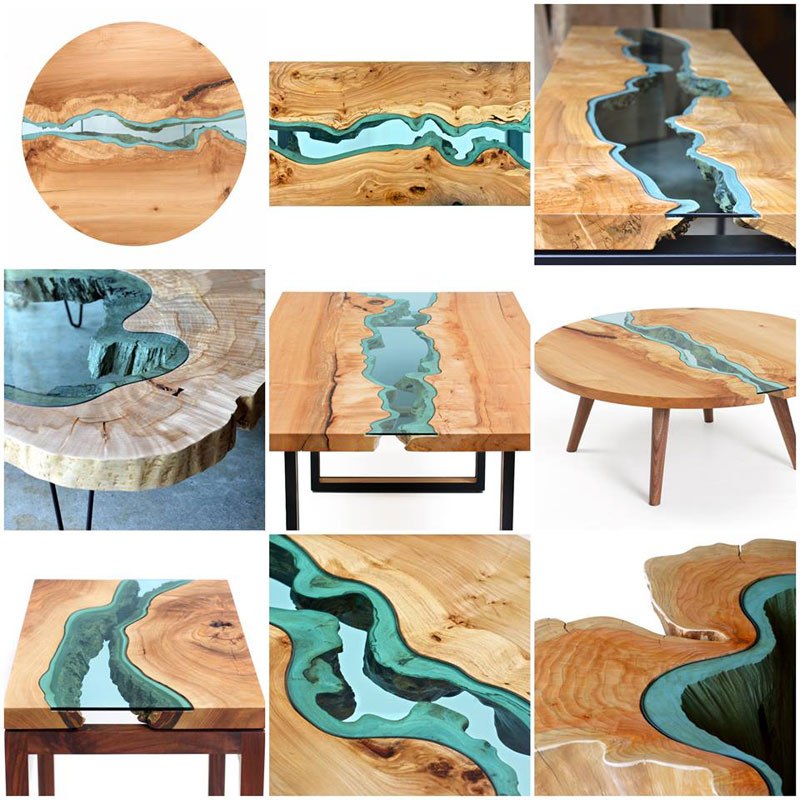
Reuben Wu – Glowing Geometric Light Paintings
Read more: Reuben Wu – Glowing Geometric Light Paintingswww.thisiscolossal.com/2021/04/reuben-wu-ex-stasis/
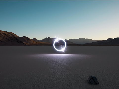
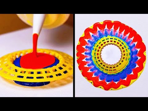
Wu programmed a stick of 200 LED lights to shift in color and shape above the calm landscapes. He captured the mesmerizing movements in-camera, and through a combination of stills, timelapse, and real-time footage, produced four audiovisual works that juxtapose the natural scenery with the artificially produced light and electronic sounds.


COLOR
-
Victor Perez – ACES Color Management in DaVinci Resolve
Read more: Victor Perez – ACES Color Management in DaVinci Resolvehttpv://www.youtube.com/watch?v=i–TS88-6xA


LIGHTING
-
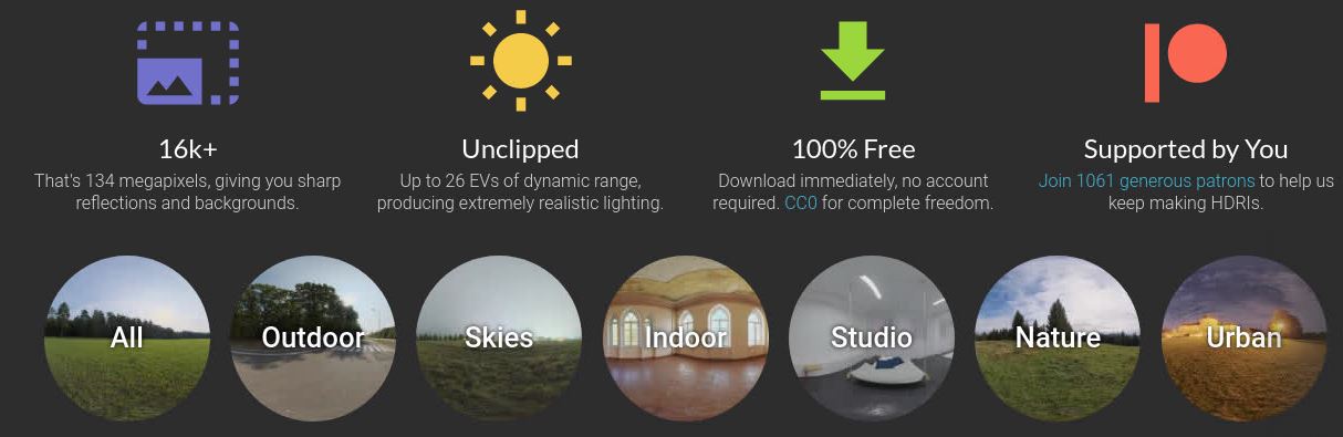
Free HDRI libraries
Read more: Free HDRI librariesnoahwitchell.com
http://www.noahwitchell.com/freebieslocationtextures.com
https://locationtextures.com/panoramas/maxroz.com
https://www.maxroz.com/hdri/listHDRI Haven
https://hdrihaven.com/Poly Haven
https://polyhaven.com/hdrisDomeble
https://www.domeble.com/IHDRI
https://www.ihdri.com/HDRMaps
https://hdrmaps.com/NoEmotionHdrs.net
http://noemotionhdrs.net/hdrday.htmlOpenFootage.net
https://www.openfootage.net/hdri-panorama/HDRI-hub
https://www.hdri-hub.com/hdrishop/hdri.zwischendrin
https://www.zwischendrin.com/en/browse/hdriLonger list here:
https://cgtricks.com/list-sites-free-hdri/
-
studiobinder.com – What is Tenebrism and Hard Lighting — The Art of Light and Shadow and chiaroscuro Explained
Read more: studiobinder.com – What is Tenebrism and Hard Lighting — The Art of Light and Shadow and chiaroscuro Explainedhttps://www.studiobinder.com/blog/what-is-tenebrism-art-definition/
https://www.studiobinder.com/blog/what-is-hard-light-photography/


-
Cinematographers Blueprint 300dpi poster
Read more: Cinematographers Blueprint 300dpi posterThe 300dpi digital poster is now available to all PixelSham.com subscribers.

If you have already subscribed and wish a copy, please send me a note through the contact page.
-
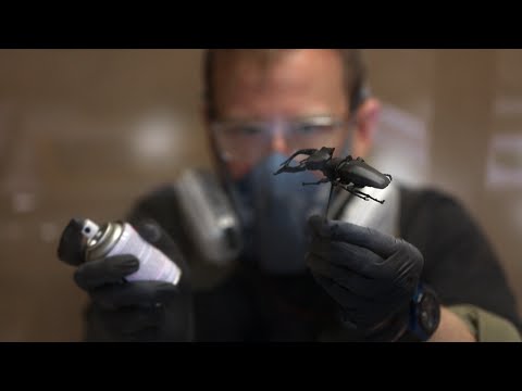
IES Light Profiles and editing software
Read more: IES Light Profiles and editing softwarehttp://www.derekjenson.com/3d-blog/ies-light-profiles
https://ieslibrary.com/en/browse#ies
https://leomoon.com/store/shaders/ies-lights-pack
https://docs.arnoldrenderer.com/display/a5afmug/ai+photometric+light
IES profiles are useful for creating life-like lighting, as they can represent the physical distribution of light from any light source.
The IES format was created by the Illumination Engineering Society, and most lighting manufacturers provide IES profile for the lights they manufacture.


COLLECTIONS
| Featured AI
| Design And Composition
| Explore posts
POPULAR SEARCHES
unreal | pipeline | virtual production | free | learn | photoshop | 360 | macro | google | nvidia | resolution | open source | hdri | real-time | photography basics | nuke
FEATURED POSTS
-
Types of AI Explained in a few Minutes – AI Glossary
-
NVidia – High-Fidelity 3D Mesh Generation at Scale with Meshtron
-
Animation/VFX/Game Industry JOB POSTINGS by Chris Mayne
-
How do LLMs like ChatGPT (Generative Pre-Trained Transformer) work? Explained by Deep-Fake Ryan Gosling
-
4dv.ai – Remote Interactive 3D Holographic Presentation Technology and System running on the PlayCanvas engine
-
Embedding frame ranges into Quicktime movies with FFmpeg
-
Cinematographers Blueprint 300dpi poster
-
JavaScript how-to free resources
Social Links
DISCLAIMER – Links and images on this website may be protected by the respective owners’ copyright. All data submitted by users through this site shall be treated as freely available to share.
