


BREAKING NEWS
LATEST POSTS
-
FXGuide – ACES 2.0 with ILM’s Alex Fry

https://draftdocs.acescentral.com/background/whats-new/
ACES 2.0 is the second major release of the components that make up the ACES system. The most significant change is a new suite of rendering transforms whose design was informed by collected feedback and requests from users of ACES 1. The changes aim to improve the appearance of perceived artifacts and to complete previously unfinished components of the system, resulting in a more complete, robust, and consistent product.
Highlights of the key changes in ACES 2.0 are as follows:
- New output transforms, including:
- A less aggressive tone scale
- More intuitive controls to create custom outputs to non-standard displays
- Robust gamut mapping to improve perceptual uniformity
- Improved performance of the inverse transforms
- Enhanced AMF specification
- An updated specification for ACES Transform IDs
- OpenEXR compression recommendations
- Enhanced tools for generating Input Transforms and recommended procedures for characterizing prosumer cameras
- Look Transform Library
- Expanded documentation
Rendering Transform
The most substantial change in ACES 2.0 is a complete redesign of the rendering transform.
ACES 2.0 was built as a unified system, rather than through piecemeal additions. Different deliverable outputs “match” better and making outputs to display setups other than the provided presets is intended to be user-driven. The rendering transforms are less likely to produce undesirable artifacts “out of the box”, which means less time can be spent fixing problematic images and more time making pictures look the way you want.
Key design goals
- Improve consistency of tone scale and provide an easy to use parameter to allow for outputs between preset dynamic ranges
- Minimize hue skews across exposure range in a region of same hue
- Unify for structural consistency across transform type
- Easy to use parameters to create outputs other than the presets
- Robust gamut mapping to improve harsh clipping artifacts
- Fill extents of output code value cube (where appropriate and expected)
- Invertible – not necessarily reversible, but Output > ACES > Output round-trip should be possible
- Accomplish all of the above while maintaining an acceptable “out-of-the box” rendering
- New output transforms, including:
-
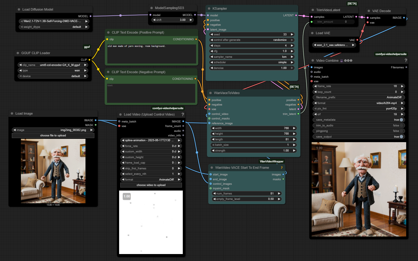
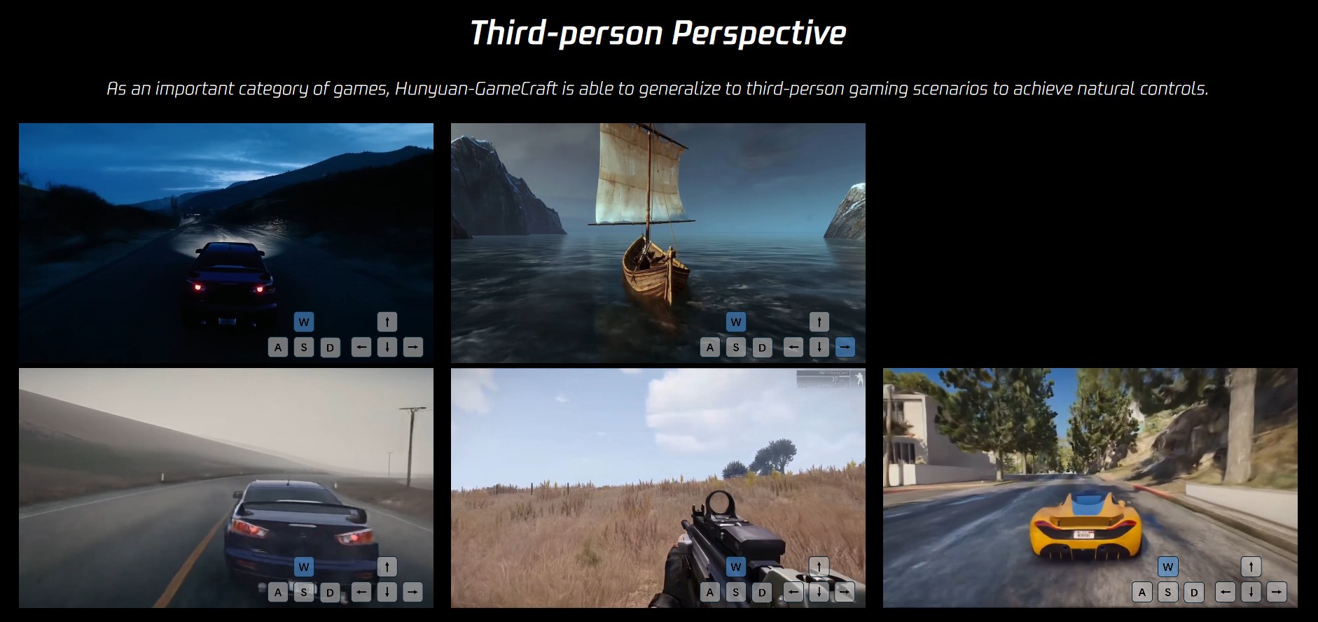
WhatDreamsCost Spline-Path-Control – Create motion controls for ComfyUI
https://github.com/WhatDreamsCost/Spline-Path-Control
https://whatdreamscost.github.io/Spline-Path-Control/
https://github.com/WhatDreamsCost/Spline-Path-Control/tree/main/example_workflows
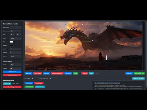
Spline Path Control is a simple tool designed to make it easy to create motion controls. It allows you to create and animate shapes that follow splines, and then export the result as a
.webmvideo file.
This project was created to simplify the process of generating control videos for tools like VACE. Use it to control the motion of anything (camera movement, objects, humans etc) all without extra prompting.- Multi-Spline Editing: Create multiple, independent spline paths
- Easy To Use Controls: Quickly edit splines and points
- Full Control of Splines and Shapes:
- Start Frame: Set a delay before a spline’s animation begins.
- Duration: Control the speed of the shape along its path.
- Easing: Apply
Linear,Ease-in,Ease-out, andEase-in-outfunctions for smooth acceleration and deceleration. - Tension: Adjust the “curviness” of the spline path.
- Shape Customization: Change the shape (circle, square, triangle), size, fill color, and border.
- Reference Images: Drag and drop or upload a background image to trace paths over an existing image.
- WebM Export: Export your animation with a white background, perfect for use as a control video in VACE.


FEATURED POSTS

-
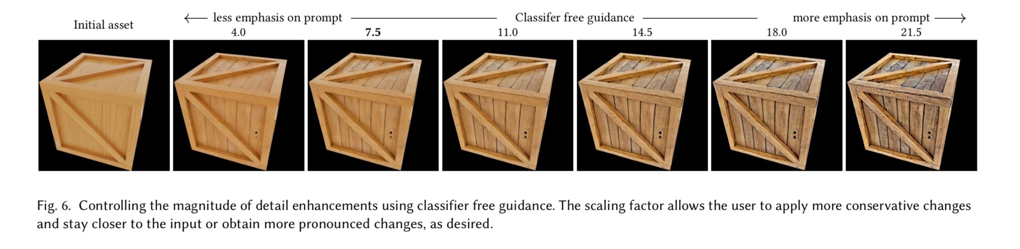
Generative Detail Enhancement for Physically Based Materials
https://arxiv.org/html/2502.13994v1
https://arxiv.org/pdf/2502.13994
A tool for enhancing the detail of physically based materials using an off-the-shelf diffusion model and inverse rendering.

-
Top 3D Printing Website Resources

The Holy Grail – https://github.com/ad-si/awesome-3d-printing
- Thingiverse – https://www.thingiverse.com/
- Makerworld – https://makerworld.com/
- Printables – https://www.printables.com/
- Cults – https://cults3d.com/
- CG Trader – https://www.cgtrader.com/3d-print-models
- Sketchfab – https://sketchfab.com/store/3d-models/stl
- 3D Export – https://3dexport.com/
- MyMiniFactory – https://www.myminifactory.com/
- Thangs – https://thangs.com/
- Yeggi – https://www.yeggi.com/
- FAB365 – https://fab365.net/
- Gambody – https://www.gambody.com/
- All3DP News – https://all3dp.com/
- TCT Magazine – https://www.tctmagazine.com/topics/3D-printing-news/
- 3DPrint.com – https://3dprint.com/
- NASA 3D Models – https://nasa3d.arc.nasa.gov/models/printable
-
Embedding frame ranges into Quicktime movies with FFmpeg
QuickTime (.mov) files are fundamentally time-based, not frame-based, and so don’t have a built-in, uniform “first frame/last frame” field you can set as numeric frame IDs. Instead, tools like Shotgun Create rely on the timecode track and the movie’s duration to infer frame numbers. If you want Shotgun to pick up a non-default frame range (e.g. start at 1001, end at 1064), you must bake in an SMPTE timecode that corresponds to your desired start frame, and ensure the movie’s duration matches your clip length.
How Shotgun Reads Frame Ranges
- Default start frame is 1. If no timecode metadata is present, Shotgun assumes the movie begins at frame 1.
- Timecode ⇒ frame number. Shotgun Create “honors the timecodes of media sources,” mapping the embedded TC to frame IDs. For example, a 24 fps QuickTime tagged with a start timecode of 00:00:41:17 will be interpreted as beginning on frame 1001 (1001 ÷ 24 fps ≈ 41.71 s).
Embedding a Start Timecode
QuickTime uses a
tmcd(timecode) track. You can bake in an SMPTE track via FFmpeg’s-timecodeflag or via Compressor/encoder settings:- Compute your start TC.
- Desired start frame = 1001
- Frame 1001 at 24 fps ⇒ 1001 ÷ 24 ≈ 41.708 s ⇒ TC 00:00:41:17
- FFmpeg example:
ffmpeg -i input.mov \
  -c copy \
  -timecode 00:00:41:17 \
  output.mov
This adds a timecode track beginning at 00:00:41:17, which Shotgun maps to frame 1001.
Ensuring the Correct End Frame
Shotgun infers the last frame from the movie’s duration. To end on frame 1064:
- Frame count = 1064 – 1001 + 1 = 64 frames
- Duration = 64 ÷ 24 fps ≈ 2.667 s
FFmpeg trim example:
ffmpeg -i input.mov \
  -c copy \
  -timecode 00:00:41:17 \
  -t 00:00:02.667 \
  output_trimmed.mov
This results in a 64-frame clip (1001→1064) at 24 fps.

-
Scientists claim to have discovered ‘new colour’ no one has seen before: Olo
https://www.bbc.com/news/articles/clyq0n3em41o
By stimulating specific cells in the retina, the participants claim to have witnessed a blue-green colour that scientists have called “olo”, but some experts have said the existence of a new colour is “open to argument”.
The findings, published in the journal Science Advances on Friday, have been described by the study’s co-author, Prof Ren Ng from the University of California, as “remarkable”.

(A) System inputs. (i) Retina map of 103 cone cells preclassified by spectral type (7). (ii) Target visual percept (here, a video of a child, see movie S1 at 1:04). (iii) Infrared cellular-scale imaging of the retina with 60-frames-per-second rolling shutter. Fixational eye movement is visible over the three frames shown.
(B) System outputs. (iv) Real-time per-cone target activation levels to reproduce the target percept, computed by: extracting eye motion from the input video relative to the retina map; identifying the spectral type of every cone in the field of view; computing the per-cone activation the target percept would have produced. (v) Intensities of visible-wavelength 488-nm laser microdoses at each cone required to achieve its target activation level.
(C) Infrared imaging and visible-wavelength stimulation are physically accomplished in a raster scan across the retinal region using AOSLO. By modulating the visible-wavelength beam’s intensity, the laser microdoses shown in (v) are delivered. Drawing adapted with permission [Harmening and Sincich (54)].
(D) Examples of target percepts with corresponding cone activations and laser microdoses, ranging from colored squares to complex imagery. Teal-striped regions represent the color “olo” of stimulating only M cones.