To measure the contrast ratio you will need a light meter. The process starts with you measuring the main source of light, or the key light.
Get a reading from the brightest area on the face of your subject. Then, measure the area lit by the secondary light, or fill light. To make sense of what you have just measured you have to understand that the information you have just gathered is in F-stops, a measure of light. With each additional F-stop, for example going one stop from f/1.4 to f/2.0, you create a doubling of light. The reverse is also true; moving one stop from f/8.0 to f/5.6 results in a halving of the light.
I was working an album cover last night and got these really cool images in midjourney so made a video out of it. Animated using Pika. Song made using Suno Full version on my bandcamp. It’s called Static.
In the retina, photoreceptors, bipolar cells, and horizontal cells work together to process visual information before it reaches the brain. Here’s how each cell type contributes to vision:
This help’s us understand the composition of components in/on solar system bodies.
Dips in the observed light spectrum, also known as, lines of absorption occur as gasses absorb energy from light at specific points along the light spectrum.
These dips or darkened zones (lines of absorption) leave a finger print which identify elements and compounds.
In this image the dark absorption bands appear as lines of emission which occur as the result of emitted not reflected (absorbed) light.
5.10 of this tool includes excellent tools to clean up cr2 and cr3 used on set to support HDRI processing.
Converting raw to AcesCG 32 bit tiffs with metadata.
About 576 megapixels for the entire field of view.
Consider a view in front of you that is 90 degrees by 90 degrees, like looking through an open window at a scene. The number of pixels would be:
90 degrees * 60 arc-minutes/degree * 1/0.3 * 90 * 60 * 1/0.3 = 324,000,000 pixels (324 megapixels).
At any one moment, you actually do not perceive that many pixels, but your eye moves around the scene to see all the detail you want. But the human eye really sees a larger field of view, close to 180 degrees. Let’s be conservative and use 120 degrees for the field of view. Then we would see:
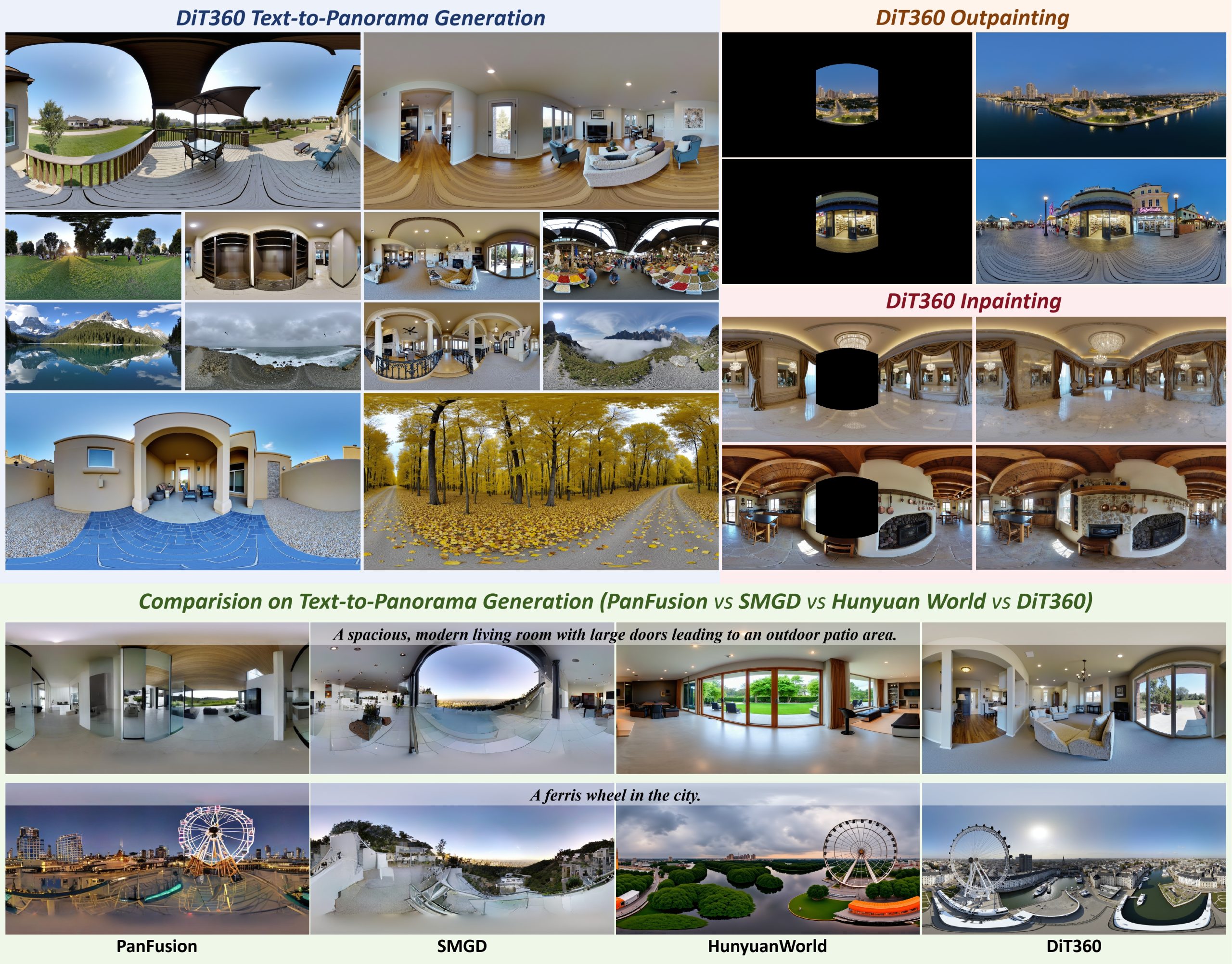
DiT360 is a framework for high-quality panoramic image generation, leveraging both perspective and panoramic data in a hybrid training scheme. It adopts a two-level strategy—image-level cross-domain guidance and token-level hybrid supervision—to enhance perceptual realism and geometric fidelity.
When collecting hdri make sure the data supports basic metadata, such as:
Iso
Aperture
Exposure time or shutter time
Color temperature
Color space Exposure value (what the sensor receives of the sun intensity in lux)
7+ brackets (with 5 or 6 being the perceived balanced exposure)
In image processing, computer graphics, and photography, high dynamic range imaging (HDRI or just HDR) is a set of techniques that allow a greater dynamic range of luminances (a Photometry measure of the luminous intensity per unit area of light travelling in a given direction. It describes the amount of light that passes through or is emitted from a particular area, and falls within a given solid angle) between the lightest and darkest areas of an image than standard digital imaging techniques or photographic methods. This wider dynamic range allows HDR images to represent more accurately the wide range of intensity levels found in real scenes ranging from direct sunlight to faint starlight and to the deepest shadows.
The two main sources of HDR imagery are computer renderings and merging of multiple photographs, which in turn are known as low dynamic range (LDR) or standard dynamic range (SDR) images. Tone Mapping (Look-up) techniques, which reduce overall contrast to facilitate display of HDR images on devices with lower dynamic range, can be applied to produce images with preserved or exaggerated local contrast for artistic effect. Photography
In photography, dynamic range is measured in Exposure Values (in photography, exposure value denotes all combinations of camera shutter speed and relative aperture that give the same exposure. The concept was developed in Germany in the 1950s) differences or stops, between the brightest and darkest parts of the image that show detail. An increase of one EV or one stop is a doubling of the amount of light.
The human response to brightness is well approximated by a Steven’s power law, which over a reasonable range is close to logarithmic, as described by the Weber�Fechner law, which is one reason that logarithmic measures of light intensity are often used as well.
HDR is short for High Dynamic Range. It’s a term used to describe an image which contains a greater exposure range than the “black” to “white” that 8 or 16-bit integer formats (JPEG, TIFF, PNG) can describe. Whereas these Low Dynamic Range images (LDR) can hold perhaps 8 to 10 f-stops of image information, HDR images can describe beyond 30 stops and stored in 32 bit images.
The intricate relationship between the eyes and the brain, often termed the eye-mind connection, reveals that vision is predominantly a cognitive process. This understanding has profound implications for fields such as design, where capturing and maintaining attention is paramount. This essay delves into the nuances of visual perception, the brain’s role in interpreting visual data, and how this knowledge can be applied to effective design strategies.
This cognitive aspect of vision is evident in phenomena such as optical illusions, where the brain interprets visual information in a way that contradicts physical reality. These illusions underscore that what we “see” is not merely a direct recording of the external world but a constructed experience shaped by cognitive processes.
Understanding the cognitive nature of vision is crucial for effective design. Designers must consider how the brain processes visual information to create compelling and engaging visuals. This involves several key principles:
DISCLAIMER – Links and images on this website may be protected by the respective owners’ copyright. All data submitted by users through this site shall be treated as freely available to share.


 Lines of emission


![[gamma correction test]](http://www.madore.org/~david/misc/color/gammatest.png "sRGB gamma correction test")