slowmoVideo is an OpenSource program that creates slow-motion videos from your footage.
Slow motion cinematography is the result of playing back frames for a longer duration than they were exposed. For example, if you expose 240 frames of film in one second, then play them back at 24 fps, the resulting movie is 10 times longer (slower) than the original filmed event….
Film cameras are relatively simple mechanical devices that allow you to crank up the speed to whatever rate the shutter and pull-down mechanism allow. Some film cameras can operate at 2,500 fps or higher (although film shot in these cameras often needs some readjustment in postproduction). Video, on the other hand, is always captured, recorded, and played back at a fixed rate, with a current limit around 60fps. This makes extreme slow motion effects harder to achieve (and less elegant) on video, because slowing down the video results in each frame held still on the screen for a long time, whereas with high-frame-rate film there are plenty of frames to fill the longer durations of time. On video, the slow motion effect is more like a slide show than smooth, continuous motion.
One obvious solution is to shoot film at high speed, then transfer it to video (a case where film still has a clear advantage, sorry George). Another possibility is to cross dissolve or blur from one frame to the next. This adds a smooth transition from one still frame to the next. The blur reduces the sharpness of the image, and compared to slowing down images shot at a high frame rate, this is somewhat of a cheat. However, there isn’t much you can do about it until video can be recorded at much higher rates. Of course, many film cameras can’t shoot at high frame rates either, so the whole super-slow-motion endeavor is somewhat specialized no matter what medium you are using. (There are some high speed digital cameras available now that allow you to capture lots of digital frames directly to your computer, so technology is starting to catch up with film. However, this feature isn’t going to appear in consumer camcorders any time soon.)
Björn Ottosson proposed OKlch in 2020 to create a color space that can closely mimic how color is perceived by the human eye, predicting perceived lightness, chroma, and hue.
The OK in OKLCH stands for Optimal Color.
L: Lightness (the perceived brightness of the color)
C: Chroma (the intensity or saturation of the color)
H: Hue (the actual color, such as red, blue, green, etc.)
In color technology, color depth also known as bit depth, is either the number of bits used to indicate the color of a single pixel, OR the number of bits used for each color component of a single pixel.
When referring to a pixel, the concept can be defined as bits per pixel (bpp).
When referring to a color component, the concept can be defined as bits per component, bits per channel, bits per color (all three abbreviated bpc), and also bits per pixel component, bits per color channel or bits per sample (bps). Modern standards tend to use bits per component, but historical lower-depth systems used bits per pixel more often.
Color depth is only one aspect of color representation, expressing the precision with which the amount of each primary can be expressed; the other aspect is how broad a range of colors can be expressed (the gamut). The definition of both color precision and gamut is accomplished with a color encoding specification which assigns a digital code value to a location in a color space.
OLED stands for Organic Light Emitting Diode. Each pixel in an OLED display is made of a material that glows when you jab it with electricity. Kind of like the heating elements in a toaster, but with less heat and better resolution. This effect is called electroluminescence, which is one of those delightful words that is big, but actually makes sense: “electro” for electricity, “lumin” for light and “escence” for, well, basically “essence.”
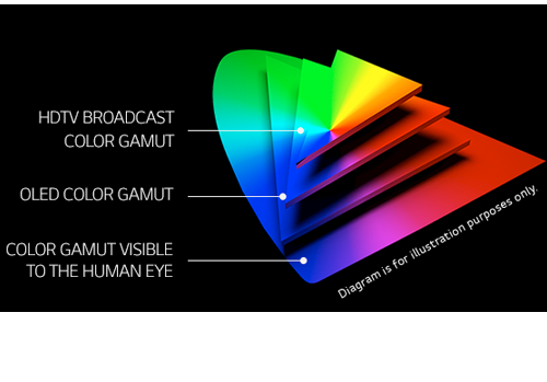
OLED TV marketing often claims “infinite” contrast ratios, and while that might sound like typical hyperbole, it’s one of the extremely rare instances where such claims are actually true. Since OLED can produce a perfect black, emitting no light whatsoever, its contrast ratio (expressed as the brightest white divided by the darkest black) is technically infinite.
OLED is the only technology capable of absolute blacks and extremely bright whites on a per-pixel basis. LCD definitely can’t do that, and even the vaunted, beloved, dearly departed plasma couldn’t do absolute blacks.
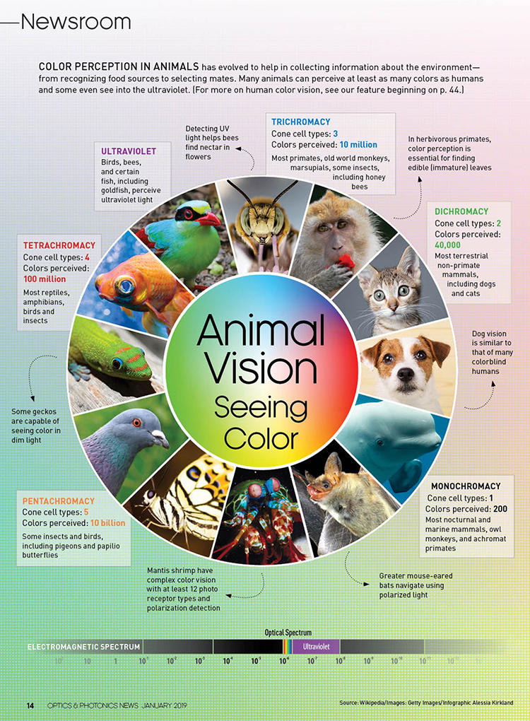
Spectral sensitivity of eye is influenced by light intensity. And the light intensity determines the level of activity of cones cell and rod cell. This is the main characteristic of human vision. Sensitivity to individual colors, in other words, wavelengths of the light spectrum, is explained by the RGB (red-green-blue) theory. This theory assumed that there are three kinds of cones. It’s selectively sensitive to red (700-630 nm), green (560-500 nm), and blue (490-450 nm) light. And their mutual interaction allow to perceive all colors of the spectrum.
Display Referred it is tied to the target hardware, as such it bakes color requirements into every type of media output request.
Scene Referred uses a common unified wide gamut and targeting audience through CDL and DI libraries instead.
So that color information stays untouched and only “transformed” as/when needed.
Sources:
– Victor Perez – Color Management Fundamentals & ACES Workflows in Nuke
– https://z-fx.nl/ColorspACES.pdf – Wicus
Most software around us today are decent at accurately displaying colors. Processing of colors is another story unfortunately, and is often done badly.
To understand what the problem is, let’s start with an example of three ways of blending green and magenta:
Perceptual blend – A smooth transition using a model designed to mimic human perception of color. The blending is done so that the perceived brightness and color varies smoothly and evenly.
Linear blend – A model for blending color based on how light behaves physically. This type of blending can occur in many ways naturally, for example when colors are blended together by focus blur in a camera or when viewing a pattern of two colors at a distance.
sRGB blend – This is how colors would normally be blended in computer software, using sRGB to represent the colors.
Let’s look at some more examples of blending of colors, to see how these problems surface more practically. The examples use strong colors since then the differences are more pronounced. This is using the same three ways of blending colors as the first example.
Instead of making it as easy as possible to work with color, most software make it unnecessarily hard, by doing image processing with representations not designed for it. Approximating the physical behavior of light with linear RGB models is one easy thing to do, but more work is needed to create image representations tailored for image processing and human perception.
One problem with sRGB is that in a gradient between blue and white, it becomes a bit purple in the middle of the transition. That’s because sRGB really isn’t created to mimic how the eye sees colors; rather, it is based on how CRT monitors work. That means it works with certain frequencies of red, green, and blue, and also the non-linear coding called gamma. It’s a miracle it works as well as it does, but it’s not connected to color perception. When using those tools, you sometimes get surprising results, like purple in the gradient.
There were also attempts to create simple models matching human perception based on XYZ, but as it turned out, it’s not possible to model all color vision that way. Perception of color is incredibly complex and depends, among other things, on whether it is dark or light in the room and the background color it is against. When you look at a photograph, it also depends on what you think the color of the light source is. The dress is a typical example of color vision being very context-dependent. It is almost impossible to model this perfectly.
I based Oklab on two other color spaces, CIECAM16 and IPT. I used the lightness and saturation prediction from CIECAM16, which is a color appearance model, as a target. I actually wanted to use the datasets used to create CIECAM16, but I couldn’t find them.
IPT was designed to have better hue uniformity. In experiments, they asked people to match light and dark colors, saturated and unsaturated colors, which resulted in a dataset for which colors, subjectively, have the same hue. IPT has a few other issues but is the basis for hue in Oklab.
In the Munsell color system, colors are described with three parameters, designed to match the perceived appearance of colors: Hue, Chroma and Value. The parameters are designed to be independent and each have a uniform scale. This results in a color solid with an irregular shape. The parameters are designed to be independent and each have a uniform scale. This results in a color solid with an irregular shape. Modern color spaces and models, such as CIELAB, Cam16 and Björn Ottosson own Oklab, are very similar in their construction.
By far the most used color spaces today for color picking are HSL and HSV, two representations introduced in the classic 1978 paper “Color Spaces for Computer Graphics”. HSL and HSV designed to roughly correlate with perceptual color properties while being very simple and cheap to compute.
Today HSL and HSV are most commonly used together with the sRGB color space.
One of the main advantages of HSL and HSV over the different Lab color spaces is that they map the sRGB gamut to a cylinder. This makes them easy to use since all parameters can be changed independently, without the risk of creating colors outside of the target gamut.
The main drawback on the other hand is that their properties don’t match human perception particularly well.
Reconciling these conflicting goals perfectly isn’t possible, but given that HSV and HSL don’t use anything derived from experiments relating to human perception, creating something that makes a better tradeoff does not seem unreasonable.
With this new lightness estimate, we are ready to look into the construction of Okhsv and Okhsl.
If you have no previous experience with Unity, start with these six video tutorials which give a quick overview of the Unity interface and some important features http://unity3d.com/support/documentation/video/
The human eye perceives half scene brightness not as the linear 50% of the present energy (linear nature values) but as 18% of the overall brightness. We are biased to perceive more information in the dark and contrast areas. A Macbeth chart helps with calibrating back into a photographic capture into this “human perspective” of the world.
In photography, painting, and other visual arts, middle gray or middle grey is a tone that is perceptually about halfway between black and white on a lightness scale in photography and printing, it is typically defined as 18% reflectance in visible light
Light meters, cameras, and pictures are often calibrated using an 18% gray card[4][5][6] or a color reference card such as a ColorChecker. On the assumption that 18% is similar to the average reflectance of a scene, a grey card can be used to estimate the required exposure of the film.
In general, when light interacts with matter, a complicated light-matter dynamic occurs. This interaction depends on the physical characteristics of the light as well as the physical composition and characteristics of the matter.
That is, some of the incident light is reflected, some of the light is transmitted, and another portion of the light is absorbed by the medium itself.
A BRDF describes how much light is reflected when light makes contact with a certain material. Similarly, a BTDF (Bi-directional Transmission Distribution Function) describes how much light is transmitted when light makes contact with a certain material
It is difficult to establish exactly how far one should go in elaborating the surface model. A truly complete representation of the reflective behavior of a surface might take into account such phenomena as polarization, scattering, fluorescence, and phosphorescence, all of which might vary with position on the surface. Therefore, the variables in this complete function would be:
incoming and outgoing angle incoming and outgoing wavelength incoming and outgoing polarization (both linear and circular) incoming and outgoing position (which might differ due to subsurface scattering) time delay between the incoming and outgoing light ray
DISCLAIMER – Links and images on this website may be protected by the respective owners’ copyright. All data submitted by users through this site shall be treated as freely available to share.


