


COMPOSITION
DESIGN
COLOR
-
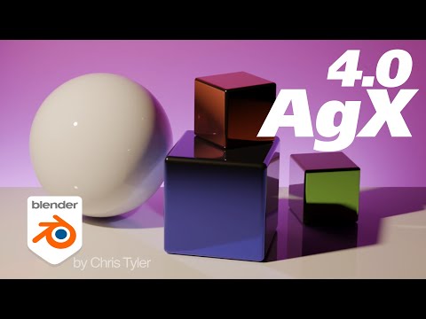
Brett Jones / Phil Reyneri (Lightform) / Philipp7pc: The study of Projection Mapping through Projectors
Read more: Brett Jones / Phil Reyneri (Lightform) / Philipp7pc: The study of Projection Mapping through Projectors


Video Projection Tool Software
https://hcgilje.wordpress.com/vpt/
https://www.projectorpoint.co.uk/news/how-bright-should-my-projector-be/
http://www.adwindowscreens.com/the_calculator/
heavym
https://heavym.net/en/
MadMapper
https://madmapper.com/
-
RawTherapee – a free, open source, cross-platform raw image and HDRi processing program
Read more: RawTherapee – a free, open source, cross-platform raw image and HDRi processing program5.10 of this tool includes excellent tools to clean up cr2 and cr3 used on set to support HDRI processing.
Converting raw to AcesCG 32 bit tiffs with metadata.


-
OpenColorIO standard
Read more: OpenColorIO standardhttps://www.provideocoalition.com/color-management-part-11-introducing-opencolorio/
OpenColorIO (OCIO) is a new open source project from Sony Imageworks.
Based on development started in 2003, OCIO enables color transforms and image display to be handled in a consistent manner across multiple graphics applications. Unlike other color management solutions, OCIO is geared towards motion-picture post production, with an emphasis on visual effects and animation color pipelines.

-
Scientists claim to have discovered ‘new colour’ no one has seen before: Olo
Read more: Scientists claim to have discovered ‘new colour’ no one has seen before: Olohttps://www.bbc.com/news/articles/clyq0n3em41o
By stimulating specific cells in the retina, the participants claim to have witnessed a blue-green colour that scientists have called “olo”, but some experts have said the existence of a new colour is “open to argument”.
The findings, published in the journal Science Advances on Friday, have been described by the study’s co-author, Prof Ren Ng from the University of California, as “remarkable”.

(A) System inputs. (i) Retina map of 103 cone cells preclassified by spectral type (7). (ii) Target visual percept (here, a video of a child, see movie S1 at 1:04). (iii) Infrared cellular-scale imaging of the retina with 60-frames-per-second rolling shutter. Fixational eye movement is visible over the three frames shown.
(B) System outputs. (iv) Real-time per-cone target activation levels to reproduce the target percept, computed by: extracting eye motion from the input video relative to the retina map; identifying the spectral type of every cone in the field of view; computing the per-cone activation the target percept would have produced. (v) Intensities of visible-wavelength 488-nm laser microdoses at each cone required to achieve its target activation level.
(C) Infrared imaging and visible-wavelength stimulation are physically accomplished in a raster scan across the retinal region using AOSLO. By modulating the visible-wavelength beam’s intensity, the laser microdoses shown in (v) are delivered. Drawing adapted with permission [Harmening and Sincich (54)].
(D) Examples of target percepts with corresponding cone activations and laser microdoses, ranging from colored squares to complex imagery. Teal-striped regions represent the color “olo” of stimulating only M cones.


LIGHTING
-
ICLight – Krea and ComfyUI light editing
Read more: ICLight – Krea and ComfyUI light editing
https://drive.google.com/drive/folders/16Aq1mqZKP-h8vApaN4FX5at3acidqPUv
https://github.com/lllyasviel/IC-Light
https://generativematte.blogspot.com/2025/03/comfyui-ic-light-relighting-exploration.html

Workflow Local copy

-
Willem Zwarthoed – Aces gamut in VFX production pdf
Read more: Willem Zwarthoed – Aces gamut in VFX production pdfhttps://www.provideocoalition.com/color-management-part-12-introducing-aces/
Local copy:
https://www.slideshare.net/hpduiker/acescg-a-common-color-encoding-for-visual-effects-applications
-
IES Light Profiles and editing software
Read more: IES Light Profiles and editing softwarehttp://www.derekjenson.com/3d-blog/ies-light-profiles
https://ieslibrary.com/en/browse#ies
https://leomoon.com/store/shaders/ies-lights-pack
https://docs.arnoldrenderer.com/display/a5afmug/ai+photometric+light
IES profiles are useful for creating life-like lighting, as they can represent the physical distribution of light from any light source.
The IES format was created by the Illumination Engineering Society, and most lighting manufacturers provide IES profile for the lights they manufacture.


-
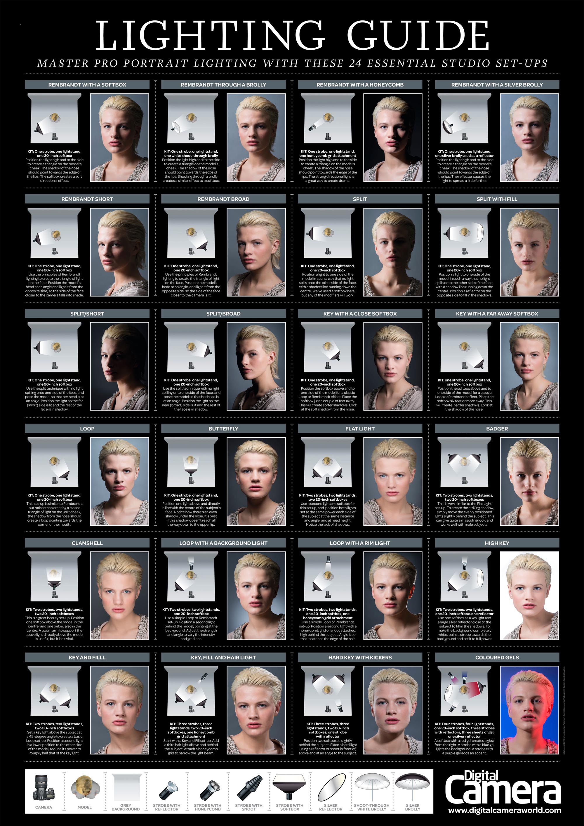
Photography basics: Why Use a (MacBeth) Color Chart?
Read more: Photography basics: Why Use a (MacBeth) Color Chart?Start here: https://www.pixelsham.com/2013/05/09/gretagmacbeth-color-checker-numeric-values/
https://www.studiobinder.com/blog/what-is-a-color-checker-tool/


In LightRoom

in Final Cut

in Nuke
Note: In Foundry’s Nuke, the software will map 18% gray to whatever your center f/stop is set to in the viewer settings (f/8 by default… change that to EV by following the instructions below).
You can experiment with this by attaching an Exposure node to a Constant set to 0.18, setting your viewer read-out to Spotmeter, and adjusting the stops in the node up and down. You will see that a full stop up or down will give you the respective next value on the aperture scale (f8, f11, f16 etc.).One stop doubles or halves the amount or light that hits the filmback/ccd, so everything works in powers of 2.
So starting with 0.18 in your constant, you will see that raising it by a stop will give you .36 as a floating point number (in linear space), while your f/stop will be f/11 and so on.If you set your center stop to 0 (see below) you will get a relative readout in EVs, where EV 0 again equals 18% constant gray.

In other words. Setting the center f-stop to 0 means that in a neutral plate, the middle gray in the macbeth chart will equal to exposure value 0. EV 0 corresponds to an exposure time of 1 sec and an aperture of f/1.0.
This will set the sun usually around EV12-17 and the sky EV1-4 , depending on cloud coverage.
To switch Foundry’s Nuke’s SpotMeter to return the EV of an image, click on the main viewport, and then press s, this opens the viewer’s properties. Now set the center f-stop to 0 in there. And the SpotMeter in the viewport will change from aperture and fstops to EV.
-
Is a MacBeth Colour Rendition Chart the Safest Way to Calibrate a Camera?
Read more: Is a MacBeth Colour Rendition Chart the Safest Way to Calibrate a Camera?www.colour-science.org/posts/the-colorchecker-considered-mostly-harmless/
“Unless you have all the relevant spectral measurements, a colour rendition chart should not be used to perform colour-correction of camera imagery but only for white balancing and relative exposure adjustments.”
“Using a colour rendition chart for colour-correction might dramatically increase error if the scene light source spectrum is different from the illuminant used to compute the colour rendition chart’s reference values.”
“other factors make using a colour rendition chart unsuitable for camera calibration:
– Uncontrolled geometry of the colour rendition chart with the incident illumination and the camera.
– Unknown sample reflectances and ageing as the colour of the samples vary with time.
– Low samples count.
– Camera noise and flare.
– Etc…“Those issues are well understood in the VFX industry, and when receiving plates, we almost exclusively use colour rendition charts to white balance and perform relative exposure adjustments, i.e. plate neutralisation.”
-
Ethan Roffler interviews CG Supervisor Daniele Tosti
Read more: Ethan Roffler interviews CG Supervisor Daniele TostiEthan Roffler
I recently had the honor of interviewing this VFX genius and gained great insight into what it takes to work in the entertainment industry. Keep in mind, these questions are coming from an artist’s perspective but can be applied to any creative individual looking for some wisdom from a professional. So grab a drink, sit back, and enjoy this fun and insightful conversation.
Ethan
To start, I just wanted to say thank you so much for taking the time for this interview!Daniele
My pleasure.
When I started my career I struggled to find help. Even people in the industry at the time were not that helpful. Because of that, I decided very early on that I was going to do exactly the opposite. I spend most of my weekends talking or helping students. ;)Ethan
(more…)
That’s awesome! I have also come across the same struggle! Just a heads up, this will probably be the most informal interview you’ll ever have haha! Okay, so let’s start with a small introduction!


COLLECTIONS
| Featured AI
| Design And Composition
| Explore posts
POPULAR SEARCHES
unreal | pipeline | virtual production | free | learn | photoshop | 360 | macro | google | nvidia | resolution | open source | hdri | real-time | photography basics | nuke
FEATURED POSTS
Social Links
DISCLAIMER – Links and images on this website may be protected by the respective owners’ copyright. All data submitted by users through this site shall be treated as freely available to share.
